An Introduction to Computational Frontal Static Stress Analysis of a Baja Car

An Introduction to Computational Frontal Static Stress

Analysis of a Baja Car

Sanika Oturkar*, Karan Gujarathi**

*

Mechanical Department, Sinhgad College of Engineering, Pune

**

Mechanical Department, Sinhgad College of Engineering, Pune

Abstract- The Society of Automotive Engineers organizes student design competitions to inculcate in students the general practices of good Engineering. One such student design activity is the SAEINDIA BAJA event held each year in Pithampur, India the aim of which is to build an All Terrain Vehicle as per the constraints given by the organizers. The growing popularity of the compet ition coupled with the need to design safe, sturdy and sustainable ATV has led to the origin of the idea of the paper. The process of dynamic stress analysis is expensive and time consuming, and simulating the problem statement is unnecessarily tedious at an initial design stage. So it is advantageous to carry out the static stress analysis first, which offers a simplistic simulation criterion of the problem statement and requires a lower computational time. This analysis will validate the safety of the preliminary design and help the designer understand the changes that need to be incorporated in the design. The paper aims to give an introduction to this static stress analysis method using ANSYS APDL 12.0, covering topics such as impact force determination, loading points, convergence of nodes, and the mesh size dependence of generated stress.

Index Terms- SAE, ATV, Static Stress Analysis, ANSYS APDL 12.0

I. INTRODUCTION

onsidering the functional objectives and the rules laid by the SAE Baja, a preliminary design of the frame structure was developed wherein the structural members and their end connections were simply represented by their centre lines and points respectively, in a 3D environment using CATIA V5. The geometries of cross-section and end connections were ignored for simplicity. Parametric modeling was implemented to ensure that future changes could be incorporated easily. A finite element (FE) model was created using the ‘Pipe 16’ element in ANSYS, on which static analysis was performed. The next step was simulating the problem statement by choosing appropriately the material properties, cross-sectional properties, positional constraints, loading conditions and mesh element size. The analysis showcases the distribution of Von Misses stresses and the deformation of the frame members, when subjected to the applied loads. If the stress generated in the chassis members was found to be above the yield limit of the material, the existing frame was modified for a safe design. The new design was again subjected to the same analysis, and the iterations continued till the stress and deformation was within the desired limit.

II. MATERIALPROPERTIES

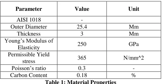
In this analysis, circular tubing of AISI 1018 having uniform cross sections was selected, confirming to the rule book. The material properties have been listed in the Table 1.

Parameter Value Unit

AISI 1018 -

Outer Diameter 25.4 Mm

Thickness 3 Mm

Young’s Modulus of

Elasticity 250 GPa

Permissible Yield

stress 365 N/mm^2

Poisson’s ratio 0.3 -

Carbon Content 0.18 %

Table 1: Material Properties

The analysis of the chassis was performed in ANSYS APDL. Node to node connectivity between members was ensured to obtain correct readings of the analysis. The line type element ‘PIPE 16’ was used. It is a uni-axial element with tension-compression, torsion and bending capabilities; and has six degrees of freedom at the two nodes: translation in the nodal X, Y, and Z directions and rotation about the nodal X, Y, and Z axes.

B. Assumptions

1) The chassis material is considered to be isotropic and homogenous. 2) Chassis tube joints are considered to be perfect joints.

3) The ‘Crumple zone’ phenomenon is not considered.

C. Calculations

1.Impact Force Determination by Speed Limit

According to the constraints in the rulebook, the maximum speed of the car is assumed to be 60km/hr or roughly around 16.66 m/s.

For a perfectly inelastic collision, the impact force is as calculated from Eqn.(1).

( )( ) ( )( ) … (1)

Where, is net work done on account of an inelastic collision.

( )( ) … (2)

… (3)

Where is the distance travelled during impact.

It is considered that for static analysis, the vehicle comes to rest 0.1 seconds after impact. Therefore, for a vehicle which moves at 16.66 m/s (or 60 km/hr), the travel of the vehicle after impact is 1.66 m. From Eqn. (1), (2) and (3), we get:

( )( ) … (4)

( )( )

Impact Force (F1) = 22990.298 N

Therefore, Impact Force by Speed Limit(F1) ≈ 23,000 N

2.Impact Force Determination by Acceleration Limit

The ‘Motor Insurance Repair Centre’ has analyzed that the baja car will see a maximum of 7.9 G’s of force during impact.

… (5)

Where, and Force = 21312.225 N

Therefore, Impact Force by Acceleration Limit (F2) ≈ 21,400 N

These two values of F1 (from Eqn.4) and F2 (from Eq. No.5) are practically comparable.

3.Impact Force Determination for Worst case Scenario

According to research, a human body will pass out at forces much higher than 7.9 G’s. Therefore, a value of 10 G’s was considered for an extreme worst case collision. Therefore for static frontal impact analysis, the load on the vehicle is calculated from Eqn. (6).

… (6)

F3 = 26,700 N

Assuming a factor of safety of 1.25 for the body frame, a force of 33,000 N is applied in the analysis.

IV. LOADINGPOINTS

The structure is loaded at the points where the Centre of gravity is located (as indicated by the yellow figures on the chassis in Fig. (1). The forces are applied on the frontal part of the chassis (as indicated by red arrows in the figure) as it is the first point of contact in case of a frontal collision.

Fig. 1

V. VON-MISSESSTRESSES

Failure of mechanical components subjected to bi-axial or tri-axial stresses occurs when the strain energy of distortion per unit volume at any point in the component, becomes equal to the strain energy of distortion per unit volume in a standard tension test specimen during yielding. According to this theory, the yield strength in shear is 0.577 times the yield strength in tension. Experiments have shown that the distortion energy theory is better in agreement for predicting the failure of ductile components than any other theory of failure.

VI. CONVERGENCENODE

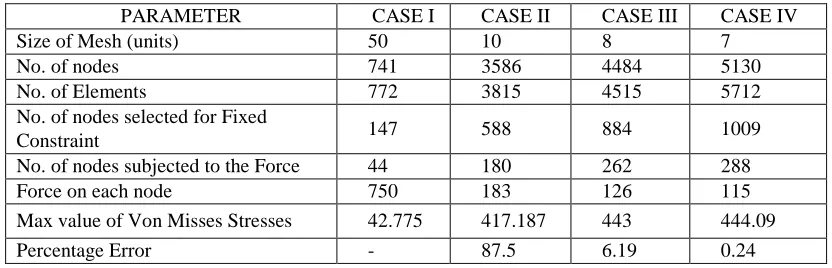
The analysis was carried out using progressively reducing elemental sizes. The elemental size having consecutive stress error less than 5% is generally considered as the optimum size of mesh. It means that any further decrease in size will only negligibly increase the accuracy of the results.

VII. OBSERVATIONTABLE

The stress values for different mesh sizes are as tabulated in Table 2.

PARAMETER CASE I CASE II CASE III CASE IV

Size of Mesh (units) 50 10 8 7

No. of nodes 741 3586 4484 5130

No. of Elements 772 3815 4515 5712

No. of nodes selected for Fixed

Constraint 147 588 884 1009

No. of nodes subjected to the Force 44 180 262 288

Force on each node 750 183 126 115

Max value of Von Misses Stresses 42.775 417.187 443 444.09

Percentage Error - 87.5 6.19 0.24

2. Two high stress regions were detected as shown in Fig. (4) and Fig. (5)

3. The maximum Von Misses stress was found to be 444.09N/mm2, which exceeds the yield strength.

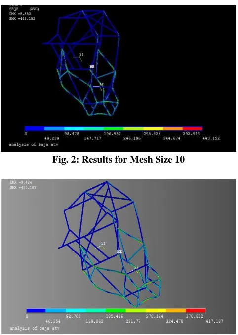
Fig. 2: Results for Mesh Size 10

Fig. 3: Results for Mesh Size 8

Fig.5: Regions of high stress concentration in Fig. 4

Fig.6: Regions of high stress concentration in Fig.4

IX. CONCLUSION

1) The analysis highlights the areas of high stress concentration, which need a change in design.

2) This preliminary analysis consumes little time and approves of a reasonable design, which can form the basis for a detailed modeled.

REFERENCES

[1] Chandrupatla, Finite Element Analysis for Engineering and Technology (University Press (India) Private Limited) [2] SAEINDIA BAJA Rule Book 2012

[3] Nagurbabu Noorbhasha, Computational Analysis for Improved Design of a SAE BAJA Frame Structure, Master of Science thesis, Howard R. Hughes College of Engineering, University of Nevada, Las Vegas, NV, December 2010

[4] ANSYS element reference digital library, ANSYS12.1

AUTHORS

First Author – Sanika Oturkar, BE Mechanical, Sinhgad College of Engineering, Pune; [email protected]

Second Author – Karan Gujarathi, BE Mechanical, Sinhgad College of Engineering, Pune; [email protected]