A Note on Price Asymmetry Using a Monetary Model

(1)

http://dx.doi.org/10.4236/tel.2014.48088

How to cite this paper: Schiaffino, P.L. and Pinasco, J.P. (2014) A Note on Price Asymmetry Using a Monetary Model. Theo-retical Economics Letters, 4, 697-701. http://dx.doi.org/10.4236/tel.2014.48088

A Note on Price Asymmetry Using a

Monetary Model

Pablo L. Schiaffino1_{, Juan Pablo Pinasco}2

1_{Facultad de Ciencias Económicas, Universidad de Palermo, Buenos Aires, Argentina} 2_{Facultad de Ciencias Exactas, Universidad de Buenos Aires, Buenos Aires, Argentina}

Email: [email protected]

Received 7 August 2014; revised 2 September 2014; accepted 8 October 2014

This work is licensed under the Creative Commons Attribution International License (CC BY). http://creativecommons.org/licenses/by/4.0/

Abstract

In this paper we present a macroeconomic foundation of downward money price inflexibility based on classical Monetary Economics. We show that under the principle of risk aversion and the neutral money axiom, our model derives an endogenous asymmetric price response as prices ad-just more rapidly when they go upward than downward. This asymmetry does not disappear; on the contrary, it is increasing in time.

Keywords

Price Asymmetry, Monetary Model, Sticky Prices, Classical Economics

1. Introduction

The literature of asymmetrical price adjustment, both theoretical and empirical, is large ([1] who offer an exten-sive comprehenexten-sive survey). For modern new Keynesian macro, the whole point was analytically to develop microfoundations to justify the existence of price asymmetry or sticky prices. Others theoretical models com-bined this microeconomic foundation with the strategic interaction factor in order to generate price asymmetries during the adjustment process [2]-[4]. Different kinds of models were built to show up price asymmetries.

(2)

698

We work with a standard Monetary model that builds on the same model that J. H. G. Olivera [5] used to study how prices adjust to its equilibrium value, but we reconstruct Olivera’s approach in order to analyze how prices behave under changes in the monetary supply. First, we show a first-order effect that the price adjustment process when the quantity of money varies is heterogeneous—a result more or less present in Olivera’s model. Second, we show a second-order effect that the initial price asymmetry tends to increase as time goes by a sim-ple but a definitely new innovation. We reconcile this result with some previous empirical and we discuss the essence of this asymmetry arguing that there is an economic intuition behind this result not only a mathematical truth.

2. The Model

The starting point is the classical conception that prices fully adjust according to money supply variations:

( ) ( ) ( ) ( )

(

, , , , , ,

)

0

p−F M p e p V p e i V i Y  = (1)

where p is the price level, p is the price time derivative, M is the nominal money supply, i is the real interest rate, e p

( )

 and V p

( )

 are the mathematical expectation and the volatility level of the price variation respectively, while e i

( )

and V i

( )

are the mathematical expectation and the volatility level of the real inter-est rate. Finally, Y is the real national income. We define F as the excess money supply function (EMSF), which according to traditional assumptions, varies positively with the nominal money supply.

The EMSF also varies negatively with the price level and positively with expected prices and price volatility. These two assumptions typically capture the reaction of money demand under expected price change and its corresponding volatility. From now on, we concentrate on money variations and its impact over the price dy-namic adjustment; hence we assume that i and Y are fixed and remain constant over time.

Proposition 1: Suppose that p=e p

( )

 and V p

( )

 is a strict increasing function of e p

( )

 . Then, if d

0 d

F

p < ;

( )

d 0 d

F

e p > ;

( )

d 0 d

F V p > ;

d 0 d

F

M > ; the immediate price reaction is asymmetrically under changes in

the quantity of money.

Proof. Recall we assume that i and Y are fixed and remain constant over time—hence, we can eliminate from (1) for the simplicity of the exposure. Also, that p=e p

( )

 and V p

( )

 is a strict increasing function of

( )

e p . Therefore, we can re-write Equation (1) into:

( )

(

, , ,

)

0

p− f M p p e p  = (2)

Let’s define an equilibrium value for price as

(

p∗,p ∗, p∗

)

. Initially, the system is in equilibrium and the

quantity of money at this point is M∗. We are interested to analyze the immediate impact of changes in the quantity of money around p∗, hence we assume that p∗= p∗ =0 tosimplify. The corresponding Taylor ap- proximation of Equation (2) can be expressed as:

(

) (

)

p=a M −M∗ +b p−p∗ +cp+d p (3)

where d

d f a

M

= ; d

d f b

p

= ; d

d f c p = ; d d f d p =

 a, c and d are positive constants while b is a negative

constant. Notice that the sign that accompanies the term d p eventually depends on the sign of p as we show in the next lines1. Equation (3) can be re-written as:

(

1−c p

)

dp =a M

(

−M∗

) (

+b p−p∗

)

(3.1) Or,

(

) (

)

(

1

)

a M M b p p

p c d ∗ ∗ − + − = − 

 (3.2)

1

The final sing over d p depends on the value of the module. That is, , 0 , 0

p p

p

p p

− <  =  _>



 

(3)

699

If prices are initially at equilibrium

(

p= p∗

)

, any movement in prices will be given by changes in the quan-tity of money supply. From here, two cases arise. The case when M >M∗, where it holds that

0

p> —recall that d 0 d

F

M > —and therefore p = p. Then,

(

)

(

1

)

a M M

p c d ∗ − = − −

 (3.3)

Conversely, when M <M∗ it holds that p<0 and p = −p :

(

)

(

1

)

a M M

p c d ∗ − = − +

 (3.4)

From Equations (3.3) and (3.4), it is immediately inferred that upward price adjustment is more rapid than downward price adjustment when the quantity of money deviates from its equilibrium value.

Proposition 2: Suppose that the same assumptions of Proposition 1 hold. Then, the price asymmetry stated in Proposition 1 is increasing in time.

Proof. The corresponding Taylor series for price at t at some t t = 0 is given by:

(

)

(

)

2

0 0 0 0 0

t t t

p= p= +p= t−t +p= t−t (4)

where at t 0 the price level is in equilibrium and equal to pt 0 p

∗

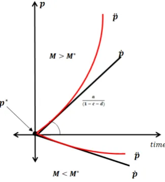
= = . Equation (4) shows that the curvature of Equation (4) depends, among other things, on the value of pt=0 (see below Figure 1). Let’s differentiate Equa-

tion (3) in order to get the second order time derivative at t0:

0 t

p=p= =aM +bp+cp+d p

    (5)

where d

d f a

M

= ; d

d f b

p

= ; d

d f c p = ; d d f d p =

 are the same constants as in Proposition 1. Similarly, the sign

that accompanies the term d p eventually depends on the sign of p and therefore, Equation (5) can be re-written using the respective parameters signs as:

(

1

)

p −c d =aM +bp

  

From here, two cases arise. The case when M >0, where it holds that p>0—recall that d 0 d

F

M > —and therefore p =p. Then,

(

1

)

aM bp p c d + = − −  _

 (5.1)

Conversely, when M <0 it holds that p<0 and p = −p:

(

1

)

aM bp p c d + = − +  _

 (5.2)

Equations (5.1) and (5.2) shows that the initial price asymmetry under changes in the quantity of money (Proposition 1) not only persists as time goes by, it also increase its magnitude when the quantity of money de-viates from its equilibrium value. Propositions 1 and 2 are resumed in Figure 1.

3. Discussion of Propositions 1 & 2

(4)

[image:4.595.233.396.86.265.2]

Figure 1. Price dynamics under changes in the quantity of money, featuring Propositions 1 & 2.

preference and its relation with volatility simply suggest that when the volatility of prices goes up, even in infla-tion or deflainfla-tion, risk-averse attitude implies a decrease in the demand for money, increasing the EMSF.

Altogether the result is described as follows. Money functions as a reserve of value and monetary actions have a quicker impact over prices compare with monetary contractions. This can be explained due to the com-

bination of the risk averse effect d

d

F

p

 

 

   and the inflation/deflation process: when money expands and infla-

tion occurs, the increase in the value of M rises the value of the price volatility; as volatility is rising, an in-creasing value for the excess money supply function (EMSF) push prices forward reinforcing the initial infla-tionary process caused initially due to the monetary expansion. When money decreases and deflation occurs, the reduction in the value of M increases price volatility and the money excess supply function. The increase in the EMSF will generate a price increase (inflation), which will offset part of the initial deflationary process due to the initial monetary contraction and, therefore, reducing volatility. For all this, positive monetary shocks will have a greater impact over prices compare with negative ones, likewise prices will react more rapidly in the up-ward case compare with the downup-ward.

4. Conclusion

This theoretical result resembles what Brandt and Wang [6] show empirically: the volatility of inflation is time-varying and tends to be high when the level of inflation is high; therefore, deflation periods will possess a lower volatility level compared to those characterized by high inflation. Since the mechanical process underling price reactions are quite different in the upward adjustment case

(

p >0

)

compared to the downward case

(

p<0

)

, under changes in the quantity of money, an asymmetry in price reactions should be expected when the quantity of money varies. This asymmetry is increasing in time, as Proposition 2 shows.

Acknowledgements

We thank Universidad de Palermo, Facultad de Ciencias Economicas for available funding. Pablo Schiaffino wishes to thank J. H.G Olivera. Much of the spirit of this note is based on the conversations that the two aca-demics hold over this particularly issue between 2011 and 2013.

References

[1] Meyer, J. and Cramon-Taubadel, S. (2004) Asymmetric Price Transmission: A Survey. Journal of Agricultural Eco-nomics, 55, 581-611. http://dx.doi.org/10.1111/j.1477-9552.2004.tb00116.x

(5)

701

Edgeworth Cycles. Econometrica: Journal of the Econometric Society, 56, 571-599. http://dx.doi.org/10.2307/1911701

[3] Sen, D. (2004) The Kinked Demand Curve Revisited. Economics Letters, 84, 99-105.

http://dx.doi.org/10.1016/j.econlet.2004.01.005

[4] Schiaffino, P. (2010) A Theory of Kinked Demand Curve: Dynamic Game Theory and Price Rigidity. Anales de la Asociación Argentina de Economía Política. http://www.aaep.org.ar/anales/works/works2010/schiaffino.pdf

[5] Olivera, J.H. (1984) Note sur l’inflexibilité des prix á la baisse. Revue d’économie politique, 94, 808-810.

(6)