ENERGY AWARE GRID RESOURCE ALLOCATION BY USING A NOVEL NEGOTIATION MODEL

ADAPTIVE NEURO FUZZY INFERENCE

SYSTEM FOR MONTHLY GROUNDWATER LEVEL

PREDICTION IN AMARAVATHI RIVER MINOR BASIN

1

G. R. UMAMAHESWARI, 2Dr. D. KALAMANI

1

Assistant Professor, Department of Mathematics, Erode Sengunthar Engineering College, Thudupathi Erode – 638 057, Tamilnadu.

2

Associate Professor, Department of Mathematics, Kongu Engineering College, Perundurai Erode – 638 052, Tamilnadu, India

E-mail: 1 [email protected] , 2 [email protected]

ABSTRACT

Adaptive Neuro Fuzzy Inference System (ANFIS) approach is employed in this present study to observe its applicability on Prediction and Forecasting of monthly Groundwater level Fluctuation in the study area (Amaravathi River Minor Basin). Study area encompasses of heavy abstraction of groundwater due to domestic, industrial and irrigation prospects which will leads in abrupt depletion of groundwater and crises on groundwater utility in future. The specific objectives are developed in the present study is to study the condition of groundwater pattern in the study area though it concern with many practical constraints. ANFI system is one of the developing powerful tools to predict such heavy constrained problem with time series analysis by hybrid technique. First part of the study is to identify the best ANFIS model which will replicate the exact behavior of groundwater system through tuning of parameters by fuzzy subset relationship and satisfying five Statistical measures (RMSE, R2, CE, COC and MBE) during training and testing processes for the duration of 2005-13. Second part of the study is to forecast the groundwater fluctuation for next one year (2014) from the identified ANFIS model.

Keywords: Groundwater Modeling, Groundwater fluctuation, ANFIS, Training, Statistical measures, RMSE, Forecasting.

1. INTRODUCTION

Groundwater is an important source for all human needs. Though the study area has regularized groundwater extraction condition, still some abrupt extractions are going on. This study, serve a primary role to predict the abrupt depletion of groundwater table by adopting ANFIS technique which doesn’t required any heavy field exploration techniques. ANFIS is associated with advanced optimization method ie., “hybrid technique” which creates a better data set relationship by neuron connection and fuzzy rules both during forwards and back propagation process.

1.1 Study Area

Amaravathi River basin is located between north latitude 110 00’ N and 100 00’ N, east longitude 770 00’ E and 780 15’ 'E. Amaravathi River is originates from Thirumurthimalai in Udumalpet taluk, Coimbatore district and flows through Erode district.

Figure 1: Groundwater Fluctuation Pattern in Amaravathi River Minor Basin (2005-13)

2. OBJECTIVES

• To develop the best ANFIS model which

will best fit to the current groundwater fluctuation pattern by hybrid technique through training and testing process after satisfying five statistical measures (Root Mean Square Value, R2, CE, COC & MSE)

• To Evaluate the prediction level of arrived

best model by comparing observed and predicted data

• To generate the possible trend of

groundwater fluctuation for next one year (2014)

3. METHODOLOGY

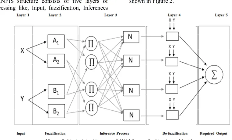
ANFIS structure consists of five layers of processing like, Input, fuzzification, Inferences

process, De-fuzzification and Required output as shown in Figure 2.

Figure 2: Typical Architecture of ANFI System for Two Input Model

ANFIS process is starts from layer 1 to layer 5. Layer 1 & 2: Input value are fuzzified, Layer 3: Inference process in which the fuzzy rules and membership function are employed for optimization of the model to get best fit, Layer

The input data for the present study are quantitative measures of groundwater fluctuation rather to language form; hence these data should be fuzzified by relative membership functions according to the real filed condition. Groundwater Recharge, Groundwater Discharge, Groundwater fluctuation level above mean sea level on monthly basis are collected from year 2005 to 2013 for the present study including the duration in which the data are collected.

Collected data are fed in to training process for the period of 2005 to 2010 (Six years), in which the hidden parameters like fuzzy sub set, rules (and/or) are framed according to the field condition. Further, testing /checking process is carried out for the period 2011 to 2013 (Three years), in which the tuned parameters are verified according to its prediction level.

Initially data are fuzzified into fuzzy subset in order to cover the whole deviation of collected data.

The subsets are defined by the seasonal variation and hydrological cycle of groundwater pattern in the study area. During data pre-processing, the data were normalized between 0 and 1 using,

xn = (xi –xmin) / (xmax – xmin),………(1) where xn is the normalized value of individual data, xi is the actual value of individual; data, xmin and xmax are the minimum and maximum values of the collected data set.

On the basis of available and collected data, the relation between fuzzy inputs and outputs are generated according to field parameter correlation; these are further used to generate fuzzy rules for the analysis. The result obtained from the analysis is in the form of a fuzzy set. This is necessarily to be de-fuzzified to get a required form output which is in the same form of available data through center of area under the curve (ie., centroid method) of de-fuzzification.

4. SENSITIVITY ANALYSIS

The process of sensitivity analysis is to find the model which can be suitable for best replication of present groundwater system by prediction the groundwater fluctuation level during training and testing process. It is essential to have such model for forecasting to next one year time series to know the expected level fluctuation at the same time, to check the condition by comparing with demand from various utility in future.

Four input and one output data analysis is carried out (Duration, Ground water discharge, Ground water recharge and monthly Groundwater level as output for the period 2005-2013) to obtain the good fitting model on the basis of five different

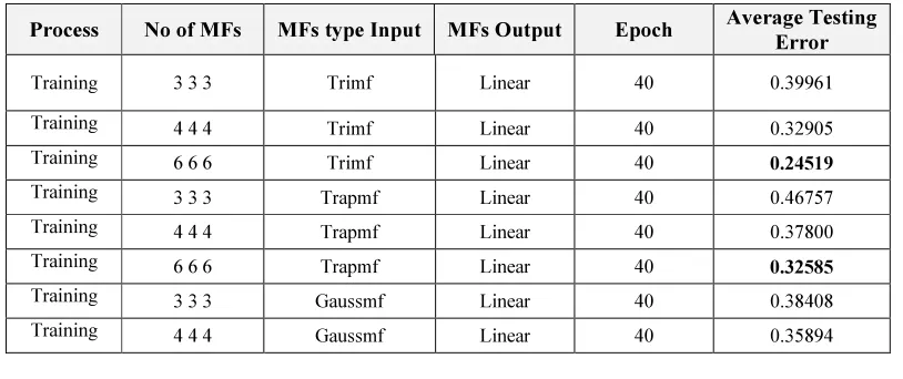
statistical measures through mamdani fuzzy inference system and hybrid optimization method. Averaging testing error produced by different Membership Functions (MF) in ANFIS model during training and testing process with constant epoch level (40) are detailed in Table 1.

From the training result, “Trimf” is performing best on the basis of low Average error emission during the training process. Further this MF is fed in to testing process to know the best fitting trend to observed value of groundwater fluctuation level. Average error produced by “Trimf” during testing process is detailed in Table 2.

Table 1: Average Training Error for Different MF for Different ANFIS Model Performance

Process No of MFs MFs type Input MFs Output Epoch Average Testing Error

Training 3 3 3 Trimf Linear 40 0.39961

Training _{4 4 4 Trimf Linear 40 0.32905}

Training _{6 6 6 Trimf Linear 40} 0.24519

Training _{3 3 3 Trapmf Linear 40 0.46757}

Training _{4 4 4 Trapmf Linear 40 0.37800}

Training _{6 6 6 Trapmf Linear 40} 0.32585

Training _{3 3 3 Gaussmf Linear 40 0.38408}

Training _{6 6 6 Gaussmf Linear 40} 0.26721

Training _{3 3 3 Gabellmf Linear 40 0.39815}

Training _{4 4 4 Gabellmf Linear 40 0.36453}

Training _{6 6 6 Gabellmf Linear} 40 0.27816

Training _{3 3 3 Gauss2mg Linear 40 0.42086}

Training _{4 4 4 Gauss2mg Linear 40 0.36733}

Training _{6 6 6 Gauss2mg Linear 40} 0.25165

Training _{3 3 3 Pimf Linear 40 0.50784}

Training _{4 4 4 Pimf Linear 40 0.36971}

Training _{6 6 6 Pimf Linear 40} 0.32583

Training _{3 3 3 dsigmf Linear 40 0.40417}

Training _{4 4 4 dsigmf Linear 40 0.35750}

Training _{6 6 6 dsigmf Linear 40} 0.24695

Training _{3 3 3 psigmf Linear 40 0.40419}

Training _{4 4 4 psigmf Linear 40 0.35746}

Training _{6 6 6 psigmf Linear} 40 0.25010

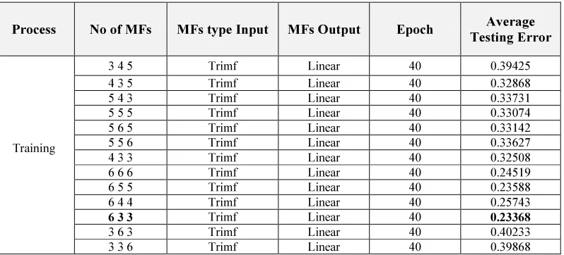
Table 2: Average Testing Error for Different MF for Different ANFIS Model Performance

Process No of MFs MFs type Input MFs Output Epoch Average

Testing Error

Training

3 4 5 Trimf Linear 40 0.39425

4 3 5 Trimf Linear 40 0.32868

5 4 3 Trimf Linear 40 0.33731

5 5 5 Trimf Linear 40 0.33074

5 6 5 Trimf Linear 40 0.33142

5 5 6 Trimf Linear 40 0.33627

4 3 3 Trimf Linear 40 0.32508

6 6 6 Trimf Linear 40 0.24519

6 5 5 Trimf Linear 40 0.23588

6 4 4 Trimf Linear 40 0.25743

6 3 3 Trimf Linear 40 0.23368

3 6 3 Trimf Linear 40 0.40233

3 3 6 Trimf Linear 40 0.39868

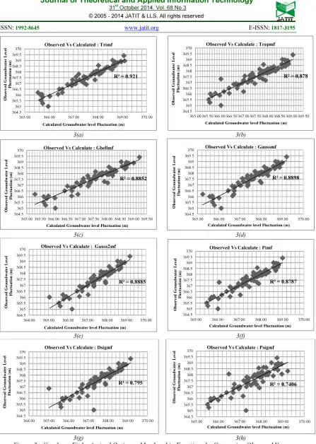
Based on the observation from sensitive analysis, ANFIS model performance is to the level of satisfactory in Triangular Membership Function at 6:3:3. More in epoch and level of rules will always lead to increase in accuracy level of prediction. The results of various ANFIS membership are detailed in Figure 3. Further the model prediction are

verified by five different statistical measure like Root mean Square error (RMSE), R-square, Coefficient of Correlation (COC), Mean Squared error (MSE) and Coefficient of Efficiency (COE) in order to obtain the optimum model which will further useful in the process of forecasting to next

3(a) 3(b)

3(c) 3(d)

3(e) 3(f)

3(g) 3(h)

Figure 3 : Goodness Fit by Arrived Optimum Membership Functions by Comparing Observed Vs Calculated { 3(a): Trimf, 3(b): Trapmf, 3(c): Gbellmf, 3(d): Gaussmf, 3(e): Gauss2mf , 3(f): Pimf,

3(g): Dsigmf, 3(h): Psigmf }

R² = 0.921

364.5 365 365.5 366 366.5 367 367.5 368 368.5 369 369.5 370

365.00 366.00 367.00 368.00 369.00 370.00

Ob se rv ed Gr o u n d wa te r L ev el F lu ct u at io n ( m )

Calculated Groundwater level Fluctuation (m) Observed Vs Calculated : Trimf

R² = 0.878

364.5 365 365.5 366 366.5 367 367.5 368 368.5 369 369.5 370

365.00 365.50 366.00 366.50 367.00 367.50 368.00 368.50 369.00 369.50

O b se rve d Gr ou n d wa te r L ev el F lu ct u at io n ( m )

Calculated Groundwater level Fluctuation (m) Observed Vs Calculate : Trapmf

R² = 0.8852

364.5 365 365.5 366 366.5 367 367.5 368 368.5 369 369.5 370

365.00 365.50 366.00 366.50 367.00 367.50 368.00 368.50 369.00 369.50

Ob se rv ed Gr ou n d wat er L eve l F lu ct u a tion ( m )

Calculated Groundwater level Fluctuation (m) Observed Vs Calculate : Gbellmf

R² = 0.8898

364.5 365 365.5 366 366.5 367 367.5 368 368.5 369 369.5 370

365.00 366.00 367.00 368.00 369.00 370.00

Ob se rve d Gr ou n d wat er L eve l F lu ct u at io n ( m )

Calculated Groundwater level Fluctuation (m) Observed Vs Calculate : Gaussmf

R² = 0.8885

364.5 365 365.5 366 366.5 367 367.5 368 368.5 369 369.5 370

364.00 365.00 366.00 367.00 368.00 369.00 370.00

Ob se rv ed Gr o u n d wat er L ev el F lu ct u at ion ( m )

Calculated Groundwater level Fluctuation (m) Observed Vs Calculate : Gauss2mf

R² = 0.8787

364.5 365 365.5 366 366.5 367 367.5 368 368.5 369 369.5 370

365.00 366.00 367.00 368.00 369.00 370.00

Ob se rve d Gr ou n d wat er L eve l F lu ct u a tion ( m )

Calculated Groundwater level Fluctuation (m) Observed Vs Calculate : Pimf

R² = 0.795

364.5 365 365.5 366 366.5 367 367.5 368 368.5 369 369.5 370

364.00 365.00 366.00 367.00 368.00 369.00 370.00

Ob se rve d Gr ou n d wat er L eve l F lu ct u a tion ( m )

Calculated Groundwater level Fluctuation (m) Observed Vs Calculate : Dsigmf

R² = 0.7406

364.5 365 365.5 366 366.5 367 367.5 368 368.5 369 369.5 370

365.00 366.00 367.00 368.00 369.00 370.00

Ob se rv ed Gr o u n d w at er L ev el F lu ct u at ion ( m )

Goodness fit analysis clearly notated the Membership Function which has comparatively more accuracy in prediction of observed value is

“Trimf”. The results obtained during other statistical measures are detailed by Radar chart is shown in Figure 4.

4(a) 4(b)

4(c) 4(d)

4(e) 4(f)

-0.2 0 0.2 0.4 0.6 0.8

1RMSE

R²

CE COC

MSE

Statistical Analysis : Trimf

-0.2 0 0.2 0.4 0.6 0.8 1

RMSE

R²

CE COC

MSE

Statistical Analysis : Trapmf

0 0.2 0.4 0.6 0.8 1

RM SE

R²

CE COC

MS E

Statistical Analysis : Gbellmf

-0.2 0 0.2 0.4 0.6 0.8 1

RMSE

R²

CE COC

MSE

Statistical Analysis : Gaussmf

-0.2 0 0.2 0.4 0.6 0.8 1

RMSE

R2

CE COC

MSE

Statistical Analysis : Gauss2mf

0 0.2 0.4 0.6 0.8 1

RM SE

R²

CE COC

MS E

4(g) 4(h)

Figure 4 : Goodness Fit by Arrived Optimum Membership Functions by Statistical Measures(Radar Chart) { 4(a): Trimf, 4(b): Trapmf, 4(c): Gbellmf, 4(d): Gaussmf, 4(e): Gauss2mf , 4(f): Pimf,

4(g): Dsigmf, 4(h): Psigmf }

5. FORECASTING

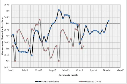
The arrived best optimum model (Trimf: 6 3 3) is used for forecasting of groundwater fluctuation to one time step (2014) as shown in Figure 5. The

result shows the decrement trend of groundwater level with the same level of groundwater recharge.

Figure 5: One Time Step Forecasting of Groundwater Fluctuation (2014) 0

0.2 0.4 0.6 0.8 1

RMSE

R²

CE COC

MSE

Statistical Analysis : Dsigmf

-0.2 0 0.2 0.4 0.6 0.8 1

RMSE

R²

CE COC

MSE

Statistical Analysis : Psigmf

364.5 365 365.5 366 366.5 367 367.5 368 368.5 369 369.5

Jan-11 Jul-11 Feb-12 Aug-12 Mar-13 Oct-13 Apr-14 Nov-14 May-15

G

r

o

u

n

d

w

a

te

r

F

lu

c

tu

a

ti

o

n

L

e

v

e

l

in

m

Duration in months

6. CONCLUSION

Based on the performance of the model, the following points are concluded.

• The proposed model is the best fit by the

hybrid technique with 6:3:3 membership function

• The sensitivity of the arrived optimum

models are satisfied under five level of statistical measures

• The forecasted model performance exactly

replicate the current situation of groundwater system

• The proposed model is further useful to

forecast under different scenario in order to develop the various management policies

REFERENCES:

[1] Alvisi .S, et. al (2006), “Water level forecasting through fuzzy logic and artificial neural network approaches”,

Hydrology and Earth System Sciences, 10,

1–17.

[2] Amir Jalalkamali & Navid Jalalkamali (2011), “Groundwater modeling using hybrid of artificial neural network with genetic algorithm”, African Journal of

Agricultural Research ,Vol. 6(26),

5775-5784

[3] Bisht D.C.S, Mohan Raju .M & Joshi M.C (2009), “Simulation of water table elevation fluctuation using fuzzy logic and ANFIS”, Computer Modelling and New

Technologies, Vol.13, No.2, 16–23

[4] Jacques W. Delleur (2007), “The Handbook of Groundwater Engineering”, Second Edition, CRC press, Taylor and Francis Group, London, 816 – 867.

[5] Kavitha Mayilvaganan .M & Naidu K.B (2011), “ANN and Fuzzy Logic models for the prediction of groundwater level of a watershed”, International Journal on

Computer Science and Engineering

(IJCSE), Vol. 3 No. 6, 2523 – 2530.

[6] Lotfi A. Zadesh & Berkeley C.A ( 1999). Fuzzy logic toolbox for use with MATLAB, The Mathwork inc. 24 prime park way, Natick, 1 – 235.

[7] Rajamanickam .R & Nagan .S (2010), “Groundwater Quality Modeling of Amaravathi River Basin of Karur District”, Tamil Nadu, Using Visual Modflow, International Journal of Environmental

Sciences, Volume 1, No1, 91 -108

[8] Sivarao (2009), “GUI Based ANFIS Modeling: Back Propagation Optimization Method for CO2 Laser Machining”,

International Journal of Intelligent

Information Technology Application,