PARIS RESEARCH LABORATORY
d i g i t a l
May 1993 Hassan A¨ıt-Kaci
Andreas Podelski Seth Copen Goldstein
Order-Sorted Feature
Theory Unification
Hassan A¨ıt-Kaci
Andreas Podelski Seth Copen Goldstein
Symposium on Logic Programming, (Vancouver, BC, Canada, October 1993), edited by Dale
Miller, and published by MIT Press, Cambridge, MA. Contact addresses of authors:
Hassan A¨ıt-Kaci and Andreas Podelski
fhak,[email protected]
Digital Equipment Corporation Paris Research Laboratory 85 Avenue Victor Hugo
92500 Rueil-Malmaison, France
Seth Copen Goldstein
University of California at Berkeley Computer Science Division
EECS, Evans Hall
Berkeley, CA 94720, USA
c
Digital Equipment Corporation 1993
records. They are sorted, attributed, possibly nested, structures, ordered thanks to a subsort ordering. Sort definitions offer the functionality of classes imposing structural constraints on objects. These constraints involve variable sorting and equations among feature paths, including self-reference. Formally, sort definitions may be seen as axioms forming an OSF theory. OSF theory unification is the process of normalizing an OSF term, using sort-unfolding to enforce structural constraints imposed on sorts by their definitions. It allows objects to inherit, and thus abide by, constraints from their classes. A formal system is thus obtained that logically models record objects with recursive class definitions accommodating multiple inheritance. We show that OSF theory unification is undecidable in general. However, we propose a set of confluent normalization rules which is complete for detecting inconsistency of an object with respect to an OSF theory. These rules translate into an efficient algorithm using structure-sharing and lazy constraint-checking. Furthermore, a subset consisting of all rules but one is confluent and terminating. This yields a practical complete normalization strategy, as well as an effective compilation scheme.
R ´esum ´e
ming, inheritance, feature structure, record calculus
Acknowledgements
1.1 Motivation of problem : : : : : : : : : : : : : : : : : : : : : : : : : : : 1 1.2 Overview of our approach : : : : : : : : : : : : : : : : : : : : : : : : : 3 1.3 Relation to other work : : : : : : : : : : : : : : : : : : : : : : : : : : : 4 1.4 Organization of paper : : : : : : : : : : : : : : : : : : : : : : : : : : : 5
2 OSF Theories 5
2.1 OSF Formalism : : : : : : : : : : : : : : : : : : : : : : : : : : : : : : 5 2.2 Sort Definitions : : : : : : : : : : : : : : : : : : : : : : : : : : : : : : : 6
3 OSF Theory Unification 9
4 Conclusion 16
A A Detailed Example 17
B OSF Formalism 21
B.1 OSF Algebras : : : : : : : : : : : : : : : : : : : : : : : : : : : : : : : 21 B.2 OSF Terms : : : : : : : : : : : : : : : : : : : : : : : : : : : : : : : : : 21 B.3 OSF Clauses : : : : : : : : : : : : : : : : : : : : : : : : : : : : : : : : 23 B.4 From OSF Terms to OSF Clauses : : : : : : : : : : : : : : : : : : : : 23 B.5 OSF Unification : : : : : : : : : : : : : : : : : : : : : : : : : : : : : : 24
I think it fair to say that the preoccupation with language among anthropologists includes a concern for expressivity and style as well as lexicology and syntax... Grammatical slips, or deviations from the idioms, can be detected by everyone, even the illiterate—unless the “errors” belong to a popular dialect, in which case they are not erroneous— because some things are generally considered to be wrong and some things cannot be said.
ROBERTDARNTON, The Great Cat Massacre
1 Synopsis
Before we develop the technical details of our method, it is important that we give the reader an informal motivation, assuming no background. We also relate our work to others, and outline the organization of the remainder of the paper.
1.1 Motivation of problem
In [3], -terms were proposed as flexible record structures for logic programming. However, -terms are of wider interest. Since they are a generalization of first-order terms, and since the latter are the pervasive data structures used by symbolic programming languages, whether based on predicate or equational logic, or pattern-directed-calculus, the more flexible -terms offer an interesting alternative.
The easiest way to describe a -term is with an example. Here is a -term that may be used to denote a generic person object:
P : person(name)id(first)string; last)S : string); age)30;
spouse)person(name)id(last)S); spouse)P)).
In words: a 30 year-old person who has a name in which the first and last parts are strings, and whose spouse is a person sharing his or her last name, that latter person’s spouse being the first person in question.
This expression looks like a record structure. Like a typical record, it has field names; i.e., the symbols on the left of). We call these feature symbols. In contrast with conventional records, however, -terms can carry more information. Namely, the fields are attached to sort symbols (e.g., person, id, string, 30, etc.). These sorts may indifferently denote individual values (e.g., 30) or sets of values (e.g., person, string). In fact, values are assimilated to singleton-denoting sorts. Sorts are partially ordered so as to reflect set inclusion; e.g.,
employee<person means that all employees are persons. Finally, sharing of structure can be expressed with variables (e.g., P and S). This sharing may be circular (e.g., P).
powerful operations as first-order terms: matching (as, say, in term-rewriting systems, or ML function definitions) and unification (as, say, in Prolog, or equational narrowing). This makes them quite a more flexible data structure for symbolic programming since both operations take into account the partial-order on sorts and extensibility with features. Therefore, they can supplement first-order terms in a functional programming language or logic programming language [3, 4]. In this manner, a form of single inheritance (matching) and multiple inheritance (unification) is obtained cleanly and efficiently. Pattern-directed definition of functions or predicates will indeed be inherited along the partial order of sorts (the sort hierarchy) thanks to matching or unification.
In object-oriented programming, typically, objects do not enjoy the expressivity offered by -terms. On the other hand, they are made according to blueprints specified as class definitions. A class acts as a template, restricting the aspect of the objects that are its instances. Our intention is to conceive such a convenience for -terms and, in so doing, expand the capability of the constraining effect of classes on objects. We propose to achieve this using
sort definitions. A sort definition associates a -term structure to a sort. Intuitively, one may then see a sort as an abbreviation of a more complex structure. Hence, a sort definition specifies a template that an object of this sort must abide by, whenever it uses any part of the structure appearing in the -term defining the sort.
For example, consider the -term:1
person(name)>(last)string); spouse)>(spouse)>;
name)>(last)“smith”))):
Without sort definitions, there is no reason to expect that this structure should be incomplete, or inconsistent, as intended. Let us now define the sort person as an abbreviation of the structure:
P : person(name)id(first)string; last)S : string);
spouse)person(name)id(last)S); spouse)P)).
This definition of the sort person expresses the expectation whereby, whenever a person object has features name and spouse, these should lead to objects of sort id and person, respectively. Moreover, if the features first and last are present in the object indicated by name, then they should be of sort string. Also, if a person object had sufficient structure as to involve feature paths name:last and spouse:name:last, then these two paths should lead to the same object. And so on.
For example, with this sort definition, the person object with last name “smith” above should be made to comply with the definition template by being normalized into the term:2
X : person(name)id(last)N : “smith”); spouse)person(spouse)X;
name)id(last)N))). 1The sort symbol
>is the top of the partial order, the sort of all objects. 2In this example, it is assumed, of course, that “smith”
Note that in our approach, we do not wish to enforce the explicit presence of the complete generic structure of a sort’s definition in every object of that sort. Rather, we want to enforce the minimal restrictions that will guarantee that every object of a given sort denotes the largest possible set consistent with the sort’s definition. For instance, we could use
person(hobby)movie going) without worrying about violating the template for person since the feature hobby is not constrained by the definition of person.
This lazy inheritance of structural constraints from the class template into an object’s structure is invaluable for efficiency reasons. Indeed, if all the (possibly voluminous) template structure of a sort were to be systematically expanded into an object of this sort that uses only a tiny portion of it, space and time would be wasted. More importantly, lazy inheritance is a way to ensure termination of consistency checking. For example, the sort definition of person above is recursive, as it involves the sort person in its body. Completely expanding these sorts into their templates would go on for ever.
An incidental benefit of sort-unfolding in the context of a sort semilattice is what we call
proof memoing. Namely, once the definition of a sort for a variable X has been unfolded, and
the attached constraints proven for X, this proof is automatically and efficiently recorded by the expanded sort. The accumulation of proofs corresponds exactly to the greatest lower bound operation. Besides the evident advantage of not having to repeat computations, this memoing phenomenon accommodates expressions which otherwise would loop. Let us take a small example to illustrate this point. Lists can be specified by declaring nil and cons to be subsorts of the sort list and by defining for the sort cons the template -term cons(head)>;tail)list). Now, consider the expression X : [1jX], the circular list containing the one element 1—i.e., desugared as X : cons(head)1;tail)X). Verifying that X is a list, since it is the tail of a cons, terminates immediately on the grounds that X has already been memoized to be a cons,
and cons< list. In contrast, the semantically equivalent Prolog program with two clauses: list([])and list([HjT]):– list(T)would make the goal list(X : [1jX])loop.
1.2 Overview of our approach
In this paper we present a formal and practical solution for the problem of checking the consistency of a -term object modulo a sort hierarchy of structural class templates. We formalize the problem in first-order logic: objects as OSF constraint formulae, classes as axioms defining an OSF theory, class inheritance as testing the satisfiability of an OSF constraint in a model of the OSF theory. We call this problem OSF theory unification.
We give conditions for the existence of non-trivial models for OSF theories, and prove the undecidability of the OSF theory unification problem. We also show that failure of OSF theory unification (i.e., non-satisfiability of an OSF term modulo an OSF theory) is semi-decidable. We propose a system of ten normalization rules that is complete for detecting incompatibility of an object with respect to an OSF theory; i.e., checking non-satisfiability of a constraint in a model of the axioms. This system specifies the third Turing-complete calculus used in LIFE [2], besides the logical and the functional one.
normalization strategy consisting of repeatedly normalizing a term first with the terminating rules, and then apply, if at all necessary, the tenth rule; and (2) it provides a compilation scheme for an OSF theory since all sort definitions of the theory can be normalized with respect to the theory itself using the weak rules.
1.3 Relation to other work
Our system is unique in that it comes with a semantic foundation and constitutes the first proven correct and complete, practical algorithm for the problem of unfolding sort definitions in order-sorted feature structures.
The problem was first already addressed in [1]. A significant difference is that the method was restricted to single inheritance and was non-lazy. Operationally, it amounted to a breadth-first expansion of all sorts and was not very practical.
Concerning undecidability of OSF theory unification, a related, but different result was proven by Gert Smolka in [13]. The undecidability of our problem uses explicitly the existence of a model satisfying the sort definitions while this is overlooked in [13] (cf., also, Footnote 6). As for unfolding sort definitions, we know of two other works, both relevant to computational linguistics: that of Bob Carpenter and that of Martin Emele and R´emi Zajac. Bob Carpenter [6] proposed a simple type-checking of a system of sort definitions for feature terms that are essentially a variation of -terms. However, besides being purely operational, this system is limited to the simple case where sort definitions specify sort constraints on features alone, without feature compositions and, more importantly, without shared variables imposing coreference constraints on feature paths. On the other hand, his formalism handles partial features, while what we present works with total features. As it turns out, our system can be made to handle partial features with the addition of one simple decidable rule whose effect is to narrow the sort of a variable to intersect a feature’s domain when that feature is applied to it. Therefore, the system described in [6] is a special case of what we present here. In the recent book [7], Chapter 15 deals with “recursive type constraint systems” extending that of [1] to be of the kind we study here. He gives a complete resolution method similar to Horn clause resolution. That method differs from ours in that it is not lazy.
The work of Emele and Zajac on typed unification grammars [10] is actually quite close to what we report here. Their work is an elaboration of [1], with the assumption that features are partial. Their main contribution has been the study of clever algorithms to carry out type unfolding efficiently. In [9], Martin Emele describes an implementation that shares many insights with the method that we describe here. In particular, he uses structure-sharing to avoid much copying overhead, and whenever copying must be done, it is done such that no redundant copying is performed. However, his technique differs from ours, in that when copying is done, all the defined features of a sort are brought into the formula where it appears. Most importantly, Emele’s algorithm is not explained in formal terms, let alone proven correct. No semantics is provided, and no clear delineation is made, as our rules do, between a maximal decidable subset of cases and the complete normalization.
defined similarly as partial functions from labels to types. What corresponds to unification in our formalism is rendered there as record concatenation. In contrast to our (possibly circular) use of logical variables and unification, coreference constraints are not supported, and self-reference is handled using a special fix-point functional abstraction. Subtyping in the Cardelli style of records is checked using static inference rules that are essentially performing the kind of verification done by Carpenter’s system [6], but made more complicated by the presence of polymorphic function types. It is hence very hard to compare that trend of work and ours because of these differences in the nature, restriction, and use of records.
1.4 Organization of paper
Section 2 presents our formalization of OSF theories and recounts essential facts about them. Section 3, the crux of the paper, presents the OSF normalization system and its formal properties. We have adjoined an appendix: Section A gives a detailed example of OSF theory normalization, and Section B reintroduces the necessary OSF formalism concepts and terminology that we need.
2 OSF Theories
2.1 OSF Formalism
Let us first recall very briefly a few OSF formalism notions and notation.3 We shall use a set of sort symbolsS, equipped with partial orderand meet operation^, together with a set
Fof feature symbols. These two sets define an OSF signature and generate a set of OSF terms with the following context-free rule:
t ::= X : s(`1)t;. . .;`n)t)
where X is a variable from a setV, s is a sort inS, and`i 2F; n0. The variable X is called the term’s root variable, referred to as Root(t)for such a term t. The sort s is called the term’s root sort, or its principal sort. We shall refer to the sort of a variable V occurring in a -term t as Sortt(V), or simply Sort(V)if the term is clear from the context.
An OSF constraint is one of (1) X : s, (2) X : = X
0
, or (3) X:` : = X
0
, where X and X0 are variables inV, s is a sort inS, and`is a feature inF. An OSF clause is a set of OSF constraints (interpreted as their conjunction).
Any OSF term t is equivalently expressible as an OSF clause, denoted (t), called its dissolved form. We shall often confuse an OSF term t for its dissolved form, writing t where we mean(t). We will use a shorthand notation to express that a variable X is constrained by an OSF term t. Namely, we denote by Ct[X] the formula X
:
=Root(t)&(t)and by C 9 t[X]
the formula9Var(t)Ct[X].
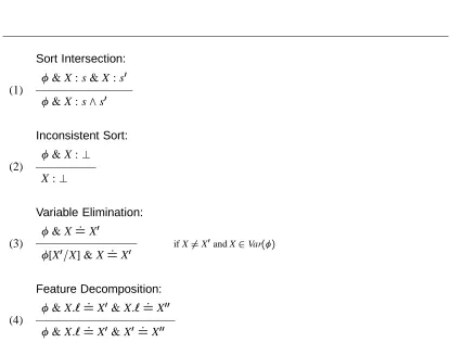
Syntactically consistent OSF terms are said to be in normal form, and called -terms. They comprise a set called . It is natural to extendand^from the sort signature to the set , where they realize matching and unification, respectively. Unification of OSF terms is done thanks to a normalization procedure. The rules to normalize OSF terms are given in Figure 1.
3The reader who is not familiar with the OSF formalism as defined in [4] will find sufficient details in appendix
Sort Intersection:
(1)
& X : s & X : s 0
& X : s^s 0
Inconsistent Sort:
(2)
& X :?
X :?
Variable Elimination:
(3)
& X : =X
0
[X 0
=X] & X : =X
0
if X6=X 0
and X2Var()
Feature Decomposition:
(4)
& X:` : =X
0 & X:`
: =X
00
& X:` : =X
0 & X0
: =X
[image:14.612.101.528.169.496.2]00
2.2 Sort Definitions
As explained in the previous section, we may view a class template as a -term. Hence, to define a sort s as a class is to associate to this sort a -term whose root sort is s. Informally, an OSF theory is a set of sort definitions, each of which is a -term whose root sort is the name of the class defined by that sort.
Formally, an OSF theory is a function:S 7! such that Sort(Root( (s)))=s for all s2S and (>)=>, (?)=?. The OSF theory = 1I
S which is the identity on Sis called the empty OSF theory.
An OSF theoryis order-consistent if it is monotonic; i.e., if8s;s 0
2S; ss 0
) (s) (s
0
). Recall that is defined on -terms (see Definition 3 on Page 22) extending the ordering on sorts.
We shall always assume the OSF theory to be order-consistent. By setting (s) = V
ss 0 (s
0
)if different from?, it is easily possible to normalize a non order-consistent theory into an equivalent order-consistent one, if it exists.
Clearly, an OSF algebra is a logical first-order structure A interpreting sort symbols as unary predicates, i.e., sets, and feature symbols as unary functions, and satisfying the axioms specified by the sort hierarchy. Namely, for all sorts s;s
0 ;s
00
such that s^s 0
=s 00
, the following axiom is valid inA:
Axiom[s^s 0
=s 00
]: 8X (X : s & X : s 0
! X : s 00
):
The name OSF theory is justified from the fact that the function specifies a system of axioms; i.e., for each s2S, the axiom:
Axiom[ (s)]:
8X X : s $ C 9 (s)
(X)
expressing that an element in the sort s necessarily satisfies the constraints attached to s (the constraints coming from the dissolved -term assigned to s by). Note that (s)contains the constraint Root( (s)): s. Thus, the equivalence($)in Axiom[
(s)]is, in fact, an implication (!).
The class of all -OSF algebras is the class of all OSF algebras such that s A
= [[ (s)]]
A
. Thus,specifies a first-order theory, namely through the system of all the axioms Axiom[s^s
0 =s
00]and Axiom
[ (s)]. The notion of
-satisfiability refers to satisfiability in a-OSF algebra; i.e., in a logical first-order structure where the axioms above hold.
We will see next that such a structure actually exists (under the overall assumption thatis order-consistent). We first define the OSF algebra 0of possibly infinite OSF graphs.
An OSF graph g= (V;E)consists of nodes denoted by mutually distinct variables inV, i.e., V V, and arcs between them, i.e., E VV. It has a distinguished node, its root, from which all its other nodes are reachable. All nodes and arcs of an OSF graph are labeled. Nodes are labeled with non-bottom sorts and arcs are labeled with feature symbols such that the same feature may not be attributed to two distinct arcs coming from the same node.
The set of all OSF graphs forms an OSF algebra:
applying the feature `to a graph g rooted in X is the maximal subgraph of g rooted in X 0 if g has an arc labeled`between nodes X and X
0
; otherwise, it is a one-node arcless graph whose node is a new distinct variable X`;glabeled with
>.
We next define the (possibly infinite) OSF clauses Unfold() obtained from an OSF clause by unfolding all sort definitions. Formally, Unfold()=
S
n0Unfoldn
(), where Unfold0()=and:
Unfoldn+1() = Unfoldn() [ fC (s)[X]
jX : s2Unfoldn()g:
We assume that the variables in the OSF constraints added to Unfoldn(), Var( (s))are new for each unfolded sort constraint X : s.
We define two formulae to be -equivalent if they are equivalent modulo the axioms specified byand the sort hierarchy and modulo existential quantification of variables in only either of the formulae. Thus,and Unfold1(), and even Unfold(), are-equivalent. The next lemma compares satisfiability ofand Unfold()in different structures.
Lemma 1 An OSF clauseis-satisfiable if and only if Unfold()is satisfiable.
Proof: Every-OSF algebra whereis satisfiable is in particular an OSF algebra where Unfold()
is satisfiable. Vice versa, the domain of an OSF algebra where Unfold()is satisfiable can be
“trimmed down” to the domain of a-OSF algebra (by including only elements which are values of
the valuations which make Unfold()hold true) such that Axiom[
(s)]holds for every sort s which
occurs in Unfold(), andis satisfiable. Sinceis order-consistent, the interpretation of the sorts
can be chosen as the restriction of the old interpretation to the new domain.
Definition 1 (Solved OSF Clauses) A (possibly infinite) OSF clauseis called solved if, for every variable X,contains:
at most one sort constraint of the form X : s, with?<s; and, at most one feature constraint of the form X:`
: =X
0
for each`;
if X : =X
0
2, then X does not appear in any other OSF constraint in.
Lemma 2 A (possibly infinite) OSF clause in solved form is satisfiable in 0, the OSF algebra of possibly infinite OSF graphs.
Proof: Let X be a variable in where X is not on the left side of the symbol :
=anywhere in.
We define the valuationon X as the graph (V;E)with the root node X, where V = S
n0 Vn,
E = S
n0
En, V0 = fXg, E0 = ;, Vn+1 = Vn [fZ j Y:` :
= Z 2 for some Y 2 Vng, En+1 = En[f(Y;Z)jY:`
:
=Z2for some Y 2Vng. A node Y is labeled by s if Y : s2for some s2S,
and by>otherwise. An arc(Y;Z)is labeled by`if Y:` : =Z2.
If X : =X
0
2, then we set(X)=(X 0
). Clearly, every OSF constraint ofholds in 0 under the
valuation.
That is, if the solved form contains X : s, then either X : s2or X 62Var(). Similarly, if it contains Y :
=X, then either Y :
=X2or Y 62Var(); and if it contains X:` :
=Y, then either X:`
:
=Y2or Y62Var().
Thus, the OSF clauseis-solved if the OSF clause:
Unfold1()=[ [
X:s2 fC
(s)[X] g
can be transformed, by applications of Rule 4, into an OSF constraint 0
of the form
0
=[1[2where1contains only equalities of the form Y :
=X where X2Var()and Y 62 Var()and2 is an OSF constraint in solved form whose variables are new for; i.e., Var()\Var(2)=;.
The OSF theory is well-formed if, for every s 2 S, the dissolved -term (s)is in
-solved form. From now on we are interested only in well-formed (and order-consistent) OSF theories.
We introduce next the OSF algebra . The domain of , and the interpretation of the features, are the ones of 0. If s2Sis a sort, then:
s
=fg2D 0
j 0;j=Unfold(X : s); (X)=gg:
In the special case of the empty theory, is the OSF graph algebra 0.
As in the case of OSF unification, i.e., of satisfiability of OSF clauses in OSF algebras, it is sufficient to consider -satisfiability in one particular-OSF algebra, here
. This characterizes as canonical
-OSF algebra (meaning: any -satisfiable OSF clause is satisfiable in ). It follows from the fact that one can easily construct a homomorphism from any-algebra into
(and, thus, is weakly final (cf., [4]) in the category of all
-OSF algebras).
Proposition 1 Given a well-formed order-consistent OSF theory, a-solved OSF clause is satisfiable in . In particular, is a
-OSF algebra, i.e., a model of the axioms specified by the sort hierarchyhS;;^iand the OSF theory.
Proof: Since, for each sort s2S, (s)is-solved, Unfoldn()is-solved, for all n. In particular,
for all n Unfoldn(), and hence also Unfold(), is-equivalent to an OSF clause in solved form.
Thus, according to Lemma 2, Unfold()is satisfiable in 0, the OSF algebra of possibly infinite
OSF graphs. Say, Unfold()holds under the valuation. Since all sort definitions in Unfold()
are unfolded, each graph g rooted in a node labeled by a sort s lies in the -denotation of s; i.e., g2s
(. . .s 0
). Thus,is in particular a
-valuation. That is, Unfold
()and, hence 0
, are satisfiable in .
3 OSF Theory Unification
We next investigate the denotational and operational semantics of the inheritance mechanism from a class template structure into an object instance. We call this mechanism OSF Theory
Unification since it is the solving of OSF clauses in the presence of an OSF theory. This
Formally, OSF Theory Unification is the procedure which-solves an OSF clause; i.e., it transformsinto a-equivalent OSF clause
0
which is either?or in-solved form (and, in this case, exhibits it).
We will show that such a procedure exists that transformssuccessively until either?or a
-solved form is obtained. Ifis-equivalent to?, then?is reachable in a finite number of steps. Generally, however, there exists no such procedure that is always terminating. Indeed, if such a procedure existed, then according to Proposition 1, there would be an algorithm deciding whether an OSF constraintis satisfiable in the-OSF algebra
. This, however, is impossible as Theorem 1 will show.
Next, we will informally describe and motivate the effect of each rule. Before doing that we need to define some additional notation. We will follow strict naming conventions for variables in order to identify them. We shall use X’s for variables appearing in a formula being normalized, and call these global or formula variables. We shall use Y’s for variables in the theory, and call these local or theory variables.
The theory variables appearing in a sort definition (s) are all local to this definition alone. Thus, without loss of generality, we shall assume distinct names for all variables across sort definitions. More precisely, s 6= s
0
) Var( (s))\Var( (s 0
)) = ;. Let Var( )=
S s2SVar
( (s))denote the set of all theory variables.
We shall use Z’s for new global variables introduced into a formula being normalized. Finally, the theory variable at the root of (s), the definition of a sort s, will be identified as Ys. We will denote by Roots( )the set of all root theory variables. Local and global variables are always assumed disjoint.
Two theory variables Y and Y0
are said to be path-compatible (noted Y +Y 0
) if they lie on the same occurrence path in the definitions where they occur. Formally, Y +Y
0
if and only if
Occ(Y)\Occ(Y 0
)6=;. 4
We will denote by`
(Y)the theory variable Y 0
, if it exists, such that `(Y)=Y 0
in some sort definition (s).
Note that Roots( )is in bijection withS. In particular, the operation^onScan be defined on Roots( )as Ys^Ys0 = Ys
^s
0. In fact, the operation ^extends homomorphically to all Var( )by defining it inductively as follows:
Y1^Y2= 8 > <
> :
Ys^s
0 if Y1
=Ysand Y2 =Ys 0;
`
(Y 0 1^Y
0
2) if Y1+Y2and Yi=`
(Y 0
i), for i=1;2;
Y? otherwise.
This operation is well-defined (1) becauseis order-consistent, and (2) thanks to the fact that path-compatible variables must lie at the end of a same feature path from their definitions’ roots and the meet (^) is defined on root variables.
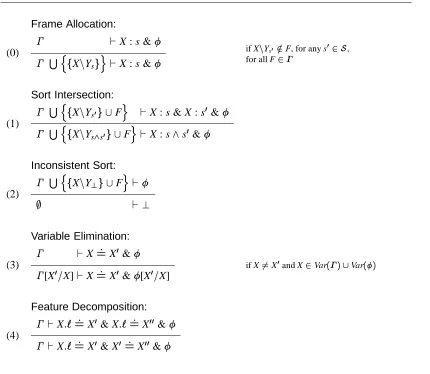
The normalization rules that perform OSF theory unification are given in Figures 2, 3, and 4 and are called OSF theory normalization rules.5 The rules in Figures 2 and 3 alone are called the weak (OSF theory) normalization rules. As for plain OSF normalization, each rule specifies a transformation of the pattern in the numerator into that of the denominator. While the rules of Figure 1 transform OSF clauses, the new rules transform contexted OSF clauses.
4See Section B for a definition of Occ.
Frame Allocation:
(0)
`X : s & S
n fXnYsg
o
`X : s &
if XnY
s0 =
2F, for any s 0
2S,
for all F2
Sort Intersection:
(1)
S n
fXnYs 0g
[F o
`X : s & X : s 0
&
S n
fXnYs ^s
0g[F o
`X : s^s 0
&
Inconsistent Sort:
(2)
S n
fXnY ?
g[F o
`
; `?
Variable Elimination:
(3)
`X : =X
0 &
[X0
=X]`X : =X
0 &[X
0 =X]
if X6=X 0
and X2Var( )[Var()
Feature Decomposition:
(4)
`X:` : =X
0 & X:`
: =X
00 &
`X:` : =X
0 & X0
: =X
[image:19.612.89.519.157.531.2]00 &
Feature Inheritance:
(5)
S n
fXnYg[F o
`X:` : =X 0 & S n
fXnY;X 0
nY 0
g[F o
`X:` : =X
0 & X0
: Sort(Y 0
)&
if`(Y)=Y 0
and X0 nY 0 = 2F Frame Merging: (6) S n
fXnYsg[F;fXnYs0g[F 0
o `
S n
fXnYs ^s
0
g[F[F 0 o ` Frame Reduction: (7) S n
fXnY;XnY 0
g[F o
`
S n
fXn(Y^Y 0
)g[F o
`
if Y+Y 0
Theory Coreference:
(8)
S n
fXnY;X 0
nYg[F o
`
S n
[image:20.612.111.521.116.395.2]fXnYg[F o `X : =X 0 &
Figure 3: Weak OSF Theory Normalization Rules—Non-Empty Theory
Theory Feature Closure:
(9)
`
`X:` :
=Z &
if XnY2F and XnY 0
2F 0
for some F;F 0
2 ,
and both`(Y),`(Y 0
)exist
(Z is a new variable)
A contexted clause is a formula of the form `whereis an OSF clause and , called the context, is a set of frames. A frame is a set of pairs of variables XnY (read “X stands for Y”) where X2Var()and Y 2Var( ). We write simplyfor;`.
The rules proceed to normalize a formula from an originally empty context, creating at most one frame per formula variable. These rules maintain frames so that there is exactly one root theory variable per frame at any moment. The global variable in a frame that stands for the root local variable is called the frame’s principal variable. Intuitively, one may think of a context as a set of activation frames, each being a local environment for a variable occurring in the formula, the pairs indicating what global variables stand for what local variables. Alternatively, one can think of a frame as the materialization of an object instance. Thus, the rules must ensure that a global variable is eventually principal in at most one frame. In addition, note that the rules will materialize only what is necessary to ensure that the instance is consistent with the class definition.
Rule (0) simply spawns a new frame for a global variable if none exists for it yet in the current context. This is akin to creating an instance in object-oriented programming. Rules (1)–(4) do exactly the same work as Rules (1)–(4) in Figure 1. The only difference is that they keep track of the sort information in the context using root theory variables. Rule (5) ensures that whenever a feature is used in the formula it fits the constraints, if any, imposed on it by the theory. Rule (6) recognizes that a global variable is principal in two frames and merges them. This case arises from variable elimination and is that of two originally distinct global variables that are later made to corefer. Rule (7) determines that the same global variable stands for two distinct path-compatible local variables within the same frame. Therefore, the global variable must stand for the common lower bound of these two local variables. Rule (8) enforces an equation of paths as prescribed by the theory when it finds that two distinct global variables stand for the same local variable in the same frame.
Rule (9) looks more complex than Rules (0)–(8). In fact, it simply completes the enforcing of functionality of features. Functionality of a feature`means that if X=X
0
then`(X)=`(X 0
). Rule (4) enforces feature functionality in the formula alone as`is applied at two occurrences of the same variable in the formula. Rule (5) does the same for the case when one occurrence is in the formula and the other is in the theory on the corresponding local variable. The only case left is when it is found that, even though a global variable is not being applied a feature` explicitly in the formula, it still may stand for two theory variables both being applied that very feature`. We need to check whether the induced equality between the two theory variables leads to an inconsistency. Therefore, a new global variable must be created and injected into the formula as the result of applying`to that global variable. This is done by an application of Rule (9). After that, Rule (5) will do the right thing, bridging the gap between the two local variables using this new global variable. In fact, it guarantees the transitivity of congruence of feature path equations as per the theory. It is this rule that may make the normalization algorithm diverge on consistent formulae as there is, in general, no way to predict how deep along a feature path an inconsistency might arise. This is indeed confirmed by the following fact.6
6A related, but different result can be found in [13] where well-formedness, order-consistency and the existence
Theorem 1 Given a well-formed order-consistent OSF theory, the problem of the satisfia-bility of an OSF constraint in the-OSF algebra
is generally undecidable.
Proof: We show that a complete OSF Theory Unification algorithm is also a decision procedure for the word problem for Thue systems of equations on strings [11]. Consider a finite alphabetand
a finite set E ?
?
of equations of words on. The word problem that consists in deciding
whether two words w1 and w2 in ?
are equal modulo the equations in E can be encoded as the following OSF theory unification problem. Let us take for sortsS = f>;s;0;1;?gwith0 <s,
1<s, and0^1 =?, and for the featuresF =. Let us definesuch that (s)is the -term
whose variables are all sorted with s and such that to each equation u=v in E corresponds one of
two occurrence paths from the root that meet in a common variable at their end.
Let us take an example to explicate this encoding. Consider the system of equations E=fbc= ed;ae=b;bd=deg. It is encoded as an OSF theory over the sorts ofSabove and the set of features F=fa;b;c;d;eg. The sort definitions are:
(s)=s(b)Y1: s(c)Y2: s;d)Y3: s); e)s(d)Y2);
a)s(e)Y1); d)s(e)Y3)):
As for (0)and (1), they both inherit the exact same structure as (s)except for the root sort since Sort(Root( (0)))=0, and Sort(Root( (1)))=1. Clearly,is a well-formed and order-consistent
OSF theory.
Now, to decide whether an equality w1=w2holds modulo the equations, it suffices to normalize the
OSF term consisting of just two non-coreferring occurrence paths w1and w2, and whose root sort is
s and all other sorts are>except for the tips of the two paths which are0and1. If the normalization
algorithm is complete, then it will necessarily make the two paths corefer (and thus end with a sort clash, i.e., normalize the dissolved -term to the equivalent OSF clause?) if and only if the equality w1 = w2 holds. Otherwise, i.e., if and only if the equality does not hold, it will normalize the
dissolved -term to an equivalent-solved OSF clause and, thus, exhibit its-satisfiability.
For example, to decide whether abc=de modulo the above equations, we need to check whether the
-term:
s(a)>(b)>(c)0)); d)>(e)1))
(i.e., the OSF clause obtained by dissolving it) is not satisfiable modulo the OSF theory given
above.
Lemma 3 If is transformed into ` 0
by the (strong) OSF theory normalization rules, thenis-equivalent to
0 .
Proof: For a contexted formula `, let us define the OSF clause:
[ `]=[ [
fC (s
)[X] & Y1 :
=X1& . . . & Yn : =Xng
of sort definitions. Thus, the result in [13] is on a test of satisfiability in all-OSF algebras, and its proof has to
where the big union is taken over the framesfXnYs;X1nY1;. . .;XnnYng2 .
The variables in C (s)[X] & Y1 :
=X1 & . . . & Yn :
=Xnare taken new for each of these frames.
Clearly,is-equivalent to [ `].
If `is transformed to 0
` 0
then [ `] is-equivalent to [ 0
` 0
]. This can be verified by inspection of each of the OSF theory normalization rules. For each application by one of these, we will give corresponding-equivalence transformations on [ `]. These will either consist of
adding C (s)[X] (again, obtained by naming its variables apart), or of applications of one of the rules
of Figure 1. Since these are all equivalence transformations, [ ` ] is equivalent, and thus also -equivalent, to [
0 `
0
].
Each application of Rule (0) of Figure 2 adds a frame fXnYsg to the context of ` . The
corresponding transformation on the OSF clause [ `] consists of adding the OSF clause C (s)[X].
One hereby obtains a-equivalent OSF clause.
Clearly, each step by application of Rule (i) of Figure 2 to ` corresponds to one step of
application of Rule (i) of Figure 1 to [ `], for i=1;. . .;4. In case of Rule (1), if s^s 0
is a strict subsort of s0
, then, in addition, C (s^s 0
)[X] has to be added.
An application of Rule (5) of Figure 3 to ` corresponds to one variable elimination step,
followed by one step of application of Rule (4) of Figure 1 (the feature constraint Y:` : =Y
0
is part of
), followed by another variable elimination step to [ `].
An application of Rule (6) of Figure 3 to ` yielding 0
` 0
corresponds to two variable elimination steps, followed by one step of application of Rule (1) of Figure 1 to [ `]. We add the
OSF clause C (s^s 0
)[X], hereby obtaining the
-equivalent OSF clause [ 0
` 0
].
An application of Rule (7) of Figure 3 corresponds to one variable elimination step, followed by one step of application of Rule (4) of Figure 1 (the feature constraints X0
:` :
=X and X 0
:` :
=Y are part of
the derived OSF clause).
An application of Rule (8) of Figure 3 corresponds to several variable elimination steps. Finally, an application of Rule (9) in Figure 4 adds a feature constraint X:`
:
=Z with a new variable Z. Clearly, [ `] is-equivalent to [ `& X:`
: =Z].
Theorem 2 Ifis transformed into the non-bottom normal form N `Nby the (strong) OSF theory normalization rules, thenNis an OSF clause in-solved form which is-equivalent to.
In particular, because we assume to be well-formed and order-consistent, is, then,
-satisfiable (e.g., in
). Of course, if
is transformed into N = ?, then is not
-satisfiable.
Proof: It is easy to see that, if N ` N is in non-bottom normal form, then [ N ` N] is in
solved form. Namely, otherwise one could apply an OSF clause normalization rule from Figure 1 to [ N ` N]; this application could, in turn, be simulated by an application of an OSF theory
normalization rule from Figure 2–4. But this means exactly thatNis in-solved form.
Proof: The number of times a sort definition is unfolded (via Rule (0)) is limited by the number of sort and of feature constraints in the OSF clause to be normalized. Let
0
is the OSF clause obtained fromby doing all these unfoldings, i.e., by adding the OSF clauses C
(s)[X], obtained by dissolving
the corresponding -terms (s)and naming its variables apart. Then, using the correspondence
from the proof of Theorem 2, each OSF theory weak normalization step oncan be simulated by an
OSF clause normalization step on 0
. Then, Theorem 7 yields the statement.
Theorem 4 The weak OSF theory normalization rules normalize a formula in almost linear time (in the size of the formula).
Proof: We use the simulation of OSF theory normalization by plain OSF clause normalization from the preceding proof and the fact that OSF clause normalization is almost linear (the size of each unfolded sort definition is assumed constant).
Theorem 5 If terminating, the (strong) OSF theory normalization rules are confluent (modulo a renaming of formula variables).
Proof: If the (strong) OSF theory normalization is terminating, Rule (9) is applied only a finite number of times. Each time, it adds a feature constraint X:`
:
=Z with a new variable Z. Letbe the
OSF clause of all these feature constraints. Then,&is transformed into the non-bottom normal
form N`Nby the weak OSF theory normalization rules only, and we can apply Theorem 3.
Theorem 6 (Completeness) If is not -satisfiable then is reduced to ? by the OSF theory normalization rules.
Proof: Using Lemma 1, ifis not-satisfiable, then Unfold()is not satisfiable.
We use the fact (which is a consequence of the compactness theorem [8]) that, given a first-order theory T and a set W of open first-order formulae, T[(9)W has a model if and only if, for every finite
subset F of W, T[(9)F has a model. Here, T is given by the axioms Axiom[s ^s
0 =s
00]and Axiom
[ (s)]
specifying the sort hierarchy and the OSF theory.
Thus, if a possibly infinite OSF clause is not satisfiable, then there exists a finite subset of it that is not satisfiable. Now, ifis not-satisfiable, then there exists an index n such that Unfoldn()is
not satisfiable. Let 0
be the minimal non-satisfiable extension ofwith sort-unfoldings, i.e., with
additions of OSF clauses of the form C (s^s 0
)[X].
According to Theorem 7, the finite OSF clause 0
is reduced to?using the OSF clause normalization
rules (1)–(4) of Figure 1. Now, every OSF clause normalization step can be simulated by an OSF theory normalization step, under the correspondence described in the proof of Theorem 2. The only difficulty is the application of the feature decomposition rule on two feature constraints which both come from sort unfoldings, i.e., from added OSF clauses of the form( (s)). In this case, the
applicability of Rule (9) has to be shown. But if follows from the fact (Theorem 3) that the weak OSF theory normalization are terminating. That is, after finitely many applications of Rules (0) to (8), none of them is applicable, and, thus, Rule (9) is.
normalization strategy. Namely, the repeated application of phase one followed by phase two. Note that if the process terminates, it terminates in phase one.
The fact that it is only Rule (9) that leads to undecidability gives us the ability to explore what makes certain theories and queries non-terminating. For instance, a loose criterion for a theory that guarantees that the normalization of all queries will terminate is that no two variables have the same feature symbols. This is clear by looking at Rule (9)’s side conditions. It is also clear that more complex, yet decidable, analysis can provide programmers using this system with this guarantee.
Another benefit of the separation is that the terminating rules can be used to “compile” a theory by using a partial evaluation technique. Namely, each sort definition can be normalized with respect to the theory using the terminating rules only.
4 Conclusion
We have presented a formal system of record objects with recursive class definitions accommodating multiple inheritance, and equational constraints among feature paths, including self-reference. Although the problem of normalizing an object to fit class templates is undecidable in general, we have proposed a complete and efficient set of rules to perform this normalization whenever it may be done.
An interesting property of this OSF theory unification process is that it consists of a terminating set of rules and an additional one which makes it complete. This property can be used to explore the exact situations when the full set of rules will be guaranteed to terminate.
Appendix
A A Detailed Example
Let us takeS =f>;s;s1;s2;s3;?gordered minimally such that s1^s2 =s3and define as:
(s1)=Ys
1 : s1(`1)Y1: s)
(s2)=Ys
2 : s2(`2)Y2: s)
(s3)=Ys
3 : s3(`1)Y3: s(`)Y4: s);`2)Y3)
(s) =Ys: s(`)Y5 : s):
The path-compatibility relation is given by Ys1 +Ys
2, Y1 + Y3, Y2 + Y3, their symmetric pairs, as well as all reflexive pairs. Therefore, the^operation is given by Ys
1^Ys 2 =Ys
3, as well as yielding the lesser element of all comparable pairs, and giving Y?otherwise.
Unifying the two -terms t1=s1(`1)s)and t2= s2(`2)s)modulo the empty theory yields the -term (up to variable renaming):
t1^ ;t2
=s3(`1)s;`2)s):
However, with respect to the theoryabove, it yields the -term (up to variable renaming):
t3=t1^ t2
as illustrated by the following reduction trace.7
7In the derivation sequence that follows, the parts of a contexted formula that make up the redex of the rule to
From empty context and initial formula:
;
` X1 : s1 & X1:`1 : =X
0
1 & X2: s2 & X2:`2 : =X
0
2 & X1
: =X2
Frame Allocation [Rule (0)] yields:
fX1nYs 1 g
` X1: s1 & X1:`1 : =X
0
1 & X2: s2 & X2:`2 : =X
0
2 & X1
: =X2
Feature Inheritance [Rule (5)] yields:
fX1nYs 1;X
0
1nY1g
` X1: s1 & X1:`1 : =X
0
1 & X0
1 : s & X2: s2 & X2:`2 : =X
0
2 & X1 : =X2
Frame Allocation [Rule (0)] yields:
fX1nYs 1;X
0
1nY1g; fX 0
1nYsg
` X1: s1 & X1:`1 : =X
0
1 & X0
1: s & X2 : s2 & X2:`2 : =X
0
2 & X1 : =X2
Frame Allocation [Rule (0)] yields:
fX1nYs 1;X
0
1nY1g; fX 0
1nYsg; fX2nYs 2 g
` X1: s1 & X1:`1 : =X
0
1 & X0
1: s & X2: s2 & X2:`2 : =X
0
2 & X1 : =X2
Feature Inheritance [Rule (5)] yields:
fX1nYs 1;X
0
1nY1g; fX 0
1nYsg; fX2nYs 2;X
0
2nY2g
` X1 : s1 & X1:`1 : =X
0
1 & X0
1: s & X2: s2 & X2:`2 : =X
0
2 & X0
2 : s
& X1 : =X2
Frame Allocation [Rule (0)] yields:
fX1nYs 1;X
0
1nY1g; fX 0
1nYsg; fX2nYs 2;X
0
2nY2g; fX 0
2nYsg
` X1 : s1 & X1:`1 : =X
0
1 & X0
1: s & X2: s2 & X2:`2 : =X
0
2 & X0
2: s
& X1 : =X2
Variable Elimination [Rule (3)] yields:
fX1nYs 1 ;X
0
1nY1g; fX 0
1nYsg; fX1nYs 2;X
0
2nY2g; fX 0
2nYsg
` X1: s1 & X1:`1 : =X
0
1 & X0
1: s & X1 : s2 & X1:`2 : =X
0
2 & X0
2: s
& X1 : =X2
Sort Intersection [Rule (1)] yields:
fX1nYs 3;X
0
1nY1g;fX 0
1nYsg; fX1nYs 2;X
0
2nY2g;fX 0
2nYsg
` X1: s3 & X1:`1 : =X
0
1 & X0
1: s & X1:`2 : =X
0
2 & X0
2: s & X1
: =X2
fX1nYs 3;X
0
1nY1;X 0
2nY2g; fX 0
1nYsg; fX 0
2nYsg
` X1: s3 & X1:`1 : =X
0
1 & X0
1: s & X1:`2 : =X
0
2 & X0
2: s & X1
: =X2
Feature Inheritance [Rule (5)] yields:
fX1nYs 3;X
0
1nY3;X 0
1nY1;X 0
2nY2g; fX 0
1nYsg; fX 0
2nYsg
` X1: s3 & X1:`1 : =X
0
1 & X0
1: s & X0
1: s & X1:`2 : =X
0
2 & X0
2: s
& X1 : =X2
Sort Intersection [Rule (1)] yields:
fX1nYs 3; X
0
1nY3 ; X 0
1nY1;X 0
2nY2g; fX 0
1nYsg; fX 0
2nYsg
` X1: s3 & X1:`1 : =X
0
1 & X0
1: s & X1:`2 : =X
0
2 & X0
2: s & X1
: =X2
Frame Reduction [Rule (7)] yields:
fX1nYs 3;X
0
1nY3;X 0
2nY2g; fX 0
1nYsg; fX 0
2nYsg
` X1: s3 & X1:`1 : =X
0
1 & X0
1: s & X1:`2 : =X
0
2 & X0
2: s & X1 : =X2
Feature Inheritance [Rule (5)] yields:
fX1nYs 3;X
0
1nY3;X 0
2nY3;X 0
2nY2g; fX 0
1nYsg; fX 0
2nYs g
` X1: s3 & X1:`1 : =X
0
1 & X0
1 : s & X1:`2 : =X
0
2 & X0
2: s & X0
2: s
& X1 : =X2
Sort Intersection [Rule (1)] yields:
fX1nYs 3;X
0
1nY3; X 0
2nY3; X 0
2nY2 g; fX 0
1nYsg; fX 0
2nYsg
` X1: s3 & X1:`1 : =X
0
1 & X0
1: s & X1:`2 : =X
0
2 & X0
2: s & X1 : =X2
Frame Reduction [Rule (7)] yields:
fX1nYs 3; X
0
1nY3 ; X 0
2nY3g; fX 0
1nYsg; fX 0
2nYsg
` X1: s3 & X1:`1 : =X
0
1 & X0
1: s & X1:`2 : =X
0
2 & X0
2: s & X1 : =X2
Theory Coreference [Rule (8)] yields:
fX1nYs 3;X
0
1nY3g; fX 0
1nYsg; fX 0
2nYsg
` X1: s3 & X1:`1 : =X
0
1 & X0
1 : s & X1:`2 : =X
0
2 & X0
2: s & X1 : =X2
& X0
1
: =X
0
2
Variable Elimination [Rule (3)] yields:
fX1nYs 3;X
0
1nY3g; fX 0
1nYsg; fX 0
1nYsg
` X1: s3 & X1:`1 : =X
0
1 & X0
1: s & X1:`2 : =X
0
1 & X0
1: s & X1 : =X2
& X0
1
: =X
0
2
fX1nYs 3;X
0
1nY3g; fX 0
1nYsg; fX 0
1nYsg
` X1: s3 & X1:`1 : =X
0
1 & X0
1: s & X1:`2 : =X
0
1 & X1
:
=X2 & X 0 1 : =X 0 2
Frame Merging [Rule (6)] yields:
fX1nYs 3; X
0
1nY3 g; fX 0
1nYsg
` X1: s3 & X1:`1 : =X
0
1 & X0
1: s & X1:`2 : =X
0
1 & X1
:
=X2 & X 0 1 : =X 0 2
Theory Feature Closure [Rule (9)] yields:
fX1nYs 3; X
0
1nY3 g; fX 0
1nYsg
` X1 : s3 & X1:`1 : =X
0
1 & X0
1: s & X1:`2 : =X
0
1 & X0
1:` :
=Z & X1 : =X2
& X0
1
: =X
0
2
Feature Inheritance [Rule (5)] yields:
fX1nYs 3;X
0
1nY3;ZnY4g; fX 0
1nYs g
` X1 : s3 & X1:`1 : =X
0
1 & X0
1: s & X1:`2 : =X
0
1 & X0
1:` :
=Z & Z : s
& X1 :
=X2 & X 0 1 : =X 0 2
Feature Inheritance [Rule (5)] yields:
fX1nYs 3;X
0
1nY3;ZnY4g; fX 0
1nYs;ZnY5g
` X1 : s3 & X1:`1 : =X
0
1 & X0
1 : s & X1:`2 : =X
0
1 & X0
1:` :
=Z & Z : s
& Z : s & X1 :
=X2 & X 0 1 : =X 0 2
Frame Allocation [Rule (0)] yields:
fX1nYs 3;X
0
1nY3;ZnY4g; fX 0
1nYs;ZnY5g; fZnYsg
` X1 : s3 & X1:`1 : =X
0
1 & X0
1 : s & X1:`2 : =X
0
1 & X0
1:` :
=Z & Z : s
& Z : s & X1 :
=X2 & X 0 1 : =X 0 2
Sort Intersection [Rule (1)] yields:
fX1nYs 3;X
0
1nY3;ZnY4g; fX 0
1nYs;ZnY5g; fZnYsg
` X1 : s3 & X1:`1 : =X
0
1 & X0
1: s & X1:`2 : =X
0
1 & X0
1:` :
=Z & Z : s
& X1 :
=X2 & X 0 1 : =X 0 2
This is in (strong)-normal form, yielding the -term (up to variable renaming):
t3=t1^ t2
B OSF Formalism
B.1 OSF Algebras
An OSF Signature is given byhS;;^;Fisuch that:
Sis a set of sorts containing the sorts>and?;
is a decidable partial order onS such that?is the least and>is the greatest element;
hS;;^iis a lower semi-lattice (s^s 0
is called the greatest common subsort of s and s0 );
Fis a set of feature symbols.
Given an OSF signaturehS;;^;Fi, an OSF algebra is a structure
A=hD A
;(s A
)s 2S
;(` A
) `2F
i
such that:
D A
is a non-empty set, called the domain ofA;
for each sort symbol s in S, s A
is a subset of the domain; in particular, > A
= D A
and
? A
=;;
(s^s 0
) A
=s A
\s 0A
for two sorts s and s0 inS;
for each feature`inF,` A
is a total unary function from the domain into the domain; i.e.,
` A
: DA 7!D
A .
An OSF homomorphism : A 7! B between two OSF algebrasA and B is a function
: D A
7!D B
such that:
(`
A
(d))=` B
((d))for all d2D A
;
(s A
) s B
.
B.2 OSF Terms
An OSF term t is an expression of the form:
X : s(`1)t1;. . .;`n)tn)
where X is a variable inV, s is a sort inS ,`1;. . .;`nare features inF, n 0, t1;. . .;tnare OSF terms, and whereV is a countably infinite set of variables.
Here is an example of an OSF term (call it tperson):
X : person(name)N :>(first)F : string); name)M : id(last)S : string);
spouse)P : person(name)I : id(last)S :>); spouse)X :>)).
We shall use a lighter notation, omitting variables that are not shared, and the sort of a variable when it is>:
X : person(name)>(first)string); name)id(last)S : string);
Given a term t = X : s(`1 ) t1;. . .;`n ) tn), the variable X is called its root variable and sometimes referred to as Root(t). The set of all variables occurring in t is defined as Var(t)=fRoot(t)g[
S n i=1Var
(ti).
Given a term t as above, an OSF interpretationA, and an A-valuation :V 7! D A
, the
denotation of t is given by:
[[t]]A;
=f(X)g \ s A
\ \
1in (`
A i )
1 ([[ti]]
A; ):
Thus, for all possible valuations of the variables, [[t]]A =
S :V7!D
A[[t]] A;
:
A -term (or OSF term in normal form) is of the form =X : s(`1 ) 1;. . .;`n) n) where:
there is at most one occurrence of a variable Y in such that Y is the root variable of a non-trivial OSF term (i.e., different than Y :>);
s is a non-bottom sort inS;
`1;. . .;`nare pairwise distinct features inF, n0, 1;. . .; nare normal OSF terms.
We call the set of all -terms. For example, the OSF term,
X : person(name)id(first)string; last)S : string);
spouse)person(name)id(last)S); spouse)X))
is a normal OSF term and denotes the same set as tperson.
Definition 3 (OSF Term Subsumption) Let and 0
be two OSF terms. Then, 0
(“ is subsumed by 0
”) if and only if, for all OSF algebrasA, [[ ]] A
[[ 0
]]A .
Given a -term , the sort of a variable V 2 Var( )will sometimes be referred to as Sort (V). Given a variable V2Var( ), an occurrence path of V in is a string of features obtained by concatenating all the features from the root leading to an occurrence of V. We call Occ (V)the set of all the occurrence paths of V in . For example, if is the -term above, then Occ (X)=f";spouse:spousegand Occ (S)=fname:last;spouse:name:lastg. The subscript will often be omitted for Sort and Occ when the context is clear.
Here are a few facts about OSF terms.
OSF terms generalize first-order terms. First-order terms form a special OSF algebra where the sorts form a flat lattice and the features are (natural number) positions. Thus, the first-order term f(t1;. . .;tn), is just the -term: f(1)t1;. . .;n)tn).
All variables occurring in an OSF term are implicitly existentially quantified at the term’s outset (assuming no further outer context). As a corollary, sorts are particular (basic) OSF
terms: indeed, [[X : s]]A =s
A since
S :V7!D
A
(f(X)g \ s A
)=s A
.
An OSF term is the empty set in all interpretations if has an occurrence of a variable sorted by the empty sort?.
Dually, [[ ]] A
=D A
X : person & X:name :
=N & N :> & N:first :
=F & F : string & X:name
:
=M & M : id & M:last :
=S & S : string & X:spouse
:
=P & P : person & P:name :
=I & I : id & I :last
:
=S & S :> & P:spouse
:
[image:32.612.101.512.68.154.2]=X & X :>:
Figure 5: OSF clause form of OSF term tperson
Features are total functions. If = X : s(`1) 1;. . .;`n) n);and Z2= Var( ), then [[ ]]A
=[[X : s(`1) 1;. . .;`n) n;`) Z :>)]] A
for any feature symbol` 2F and any OSF interpretationA.
Variables denote essentially an equality among attribute compositions. For example, [[X :>(`1 ) Y : >;`2 ) Y :>)]]
A
= fd 2D A
j` A
1(d)=` A
2(d)g:This justifies our referring to variables as coreference tags.
B.3 OSF Clauses
A logical reading of an OSF term is immediate as its information content can be characterized by a simple formula. For this purpose, we need a simple clausal language as follows.
An OSF constraint is one of (1) X : s, (2) X : = X
0
, or (3) X:` : = X
0
, where X and X0 are variables inV, s is a sort inS, and`is a feature inF. An OSF clause is a set of OSF constraints (to be interpreted as their conjunction).
GivenAis an OSF algebra, an OSF clauseis satisfiable inA,A;j=, if there exists a valuation:V 7!D
A
such that, for every OSF constraint 0
in,A;j= 0
, where:
A;j=X : s if and only if (X)2s A
;
A;j=X :
=Y if and only if (X)=(Y); A;j=X:`
:
=Y if and only if ` A
((X))=(Y): B.4 From OSF Terms to OSF Clauses
We can always associate with an OSF term = X : s(`1 ) 1;. . .;`n ) n) a corresponding OSF clause( )as follows:
( )= X : s & X:`1 : =X
0
1 & . . . & X:`n : =X
0 n
&( 1) & . . . &( n)
where X0 1;. . .;X
0
nare the roots of 1;. . .; n, respectively. We say that( )is obtained from dissolving the OSF term . For example, the non-normal OSF term tperson of Section B.2 is
dissolved into the OSF clause shown in Figure 5. It has been shown that the set-theoretic denotation of an OSF term and the logical semantics of its dissolved form coincide exactly [4]:
[[ ]]A
=f(X)j2Val(A); A;j=C 9
(X)g where C [X] is shorthand for the formula X :
=Root( )&( ), and C 9