PLACEMENT AND SIZING OF DISTRIBUTED GENERATORS IN DISTRIBUTED NETWORK BASED ON LRIC AND LOAD GROWTH CONTROL

1

PLACEMENT AND SIZING OF DISTRIBUTED

GENERATORS IN DISTRIBUTED NETWORK BASED ON

LRIC AND LOAD GROWTH CONTROL

1_{PARA KALPANA,} 2_{Dr. A.LAKSHMI DEVI}

1

Student, M.Tech., Department of Electrical Engineering, SVUCE, SV UNIVERSITY, TIRUPATI, INDIA

2_{Assoc. Prof., Department of Electrical Engineering, SVUCE, SV UNIVERSITY, TIRUPATI, INDIA}

E-mail: [email protected], [email protected]

ABSTRACT

Distributed generations (DGs) play an important role in distribution networks. Among many of their merits, loss reduction and voltage profile improvement are two of them. Studies show that optimal and non-optimal sizes of DG units may lead to increase in losses and poor voltage regulation. This paper aims at determining optimal DG location and sizing. The evaluation of best-site and size for DG unit is based on Long-Run Incremental Cost indicating the forward-looking network capacity cost at each node. By comparing DG connection cost with the decrement of the network capacity cost resulting from the DG capacity, the appropriateness of DG connecting to distribution network can be determined. On this basis, a heuristic approach is applied to identify best site and size of DG to guide the connection of DG. The proposed method is tested on an IEEE 33 bus radial distribution system.

Keywords: Distributed Generation(DG), Long-Run Incremental Cost(LRIC)

1. INTRODUCTION

DG is gaining more and more attention world wide as an alternative to large scale centralized generating stations. DG is defined as any small-scale electrical power generation technology that provides electric power at or near load-site; it is either interconnected to the distribution system, directly to the customer’s facilities or both [1]. DG capacity is ranging from few kilowatts to 50 MW [2].

Many authors claim for an unique definition in order to understand the same. But the solution to the problem is not that easy [3], because

(i) DG is , in general, not power or voltage dependent

(ii) The DG technologies can be categorized as renewable and non-renewable. DG is not a synonym for renewable source

(iii) DG can be both stand alone or grid connected (iv) DG is connected to the grid either directly or

using Transformers or Power electronics. These include protection systems as well as measuring and metering devices.

(v) Geographical location is not a relevant parameter to distinguish DG from central generation

(vi) The DG benefits are environmental protection, power quality, reduction of T&D losses and investments, use of domestic fuels and diversified resources, backup and peak shaving CHP applications, network reinforcement and energy supply for remote areas, and increase of local employment

DG produces electricity near the load site. This approach is not likely to be used to replace central station plants, but it could respond to particular needs with in competitive markets. However, many observers predict an increasing share of distributed generation in competitive electricity markets. Possible growth applications are [4]:

• Industrial co-generation

• Support for network operation (provision of ancillary services)

• Insurance against power outages (standby power)

• Avoidance of high electricity prices during periods of peak demand

• Overcoming power transmission bottlenecks

2 system planning is important. Inappropriate siting and sizing of DGs could lead to many negative effects on the distribution system concerned, such as voltage profiles and network losses [6]. In this work, the site and size of DG connecting to distribution network based on economic potential for DG has been considered from the perspective of social benefit. A new method to evaluate the connection of DG is presented based on Long-Run Incremental Cost (LRIC) indicating the forward-looking capacity cost at each node. The proposed approach seeks to reflect the cost of advancing or deferring future investment consequent upon the addition of generation or load at each study node on a distribution or transmission network. For network components that support a nodal power injection or withdrawal of power, there will be an associated cost if investment is advanced, or benefit if it can be deferred. The LRIC charges are determined as the difference in the present value of the future investment with and without the nodal injection or withdrawal. LRIC reflects the incremental cost or benefits to the network.

The rest of the paper is organized as follows: section2 describes the mathematical formulation of the proposed LRIC methodology. Section 3 gives DG connection cost. Section 4 provides the algorithm to identify the optimal location and sizing of DG. Section 5 provides the test results. Section 6 gives the conclusions of the paper. Finally section 7 provides list of the references used.

2. LONG-RUN INCREMENTAL COST

LRIC is the change in cost resulting from change in demand. The LRIC of a branch is obtained as follows [7]:

If a network component k, such as a branch, has a capacity of Ck, and supports a power

flow of Pk , then the number of years it takes to

grow from Pk to Ck for a given load growth speed d

can be given by

(1

)

nk

k k k

C

=

P

+

d

(1) Rearranging the above equation

(log

log

)

log(1

)

k k k k

C

P

n

d

−

=

+

(2)

It is assumed that the reinforcement will occur when the circuit is fully loaded. Thus investment will occur in nk years when the circuit

utilization reaches Ck. At this point a duplication of

the network component is taken as the future investment. The future investment can be discounted back to its present value. If a discount

rate x is chosen, then the present value of the future investment in nk years will be

asset

x

(1+ )

k

pv k

k n

C

=

(3)

Where asset and

C

_kpv are the modern equivalent asset cost and its present value

If the power flow change along line is

k

P

∆

, then the additional withdrawn at the node is

P

∆

.This will bring the forward future investment from year

n

_k to

n

_k*.

(

)(1

)

n*k

k k P k

C

=

P

+

∆

+

d

(4)

Where

n

*_k is the new number of years to reach the branch capacity.

Rearranging the above equation

*

log

log(

)

log(1

)

k k k k P

C

P

n

d

∆

−

+

=

+

(5)

Similarly, the present value of the future investment will change to

*

*

asset

x

(1+ )

k

pv k

k _n

C

=

(6)

Where *

pv k

C

is the new present value as the result of the additional load.

Therefore, Annual incremental cost of branch k after adding ∆P load, given by [8]

*

*

pv pv k k k P

C

C

C

CRF

∆

∆

−

=

(7)

Where CRF is the capital recovery factor, which is defined as the ratio between a uniform annual value within the planning horizon and present value of the annual stream.

If ∆P is close to zero ∆Ck is the derivative

of

C

_kpv with respect to Pk. Therefore annual

increment cost of a branch k is given by equation (8)

(ln ln )/ln(1 )

ln(1

)

*

(1

)

ln(1

)

3 i i k k U

C

m

∈

∆

=

∑

(9)

Where

m

_i is the LRIC at node i, Ui is the set of

upstream buses of node i.

LRIC reflects the cost of advancing future investment consequent on the addition of unit load at each node in distribution system.

Now the capacity cost of the network can be expressed as

_MWnet _{Li i}

i S

C

P m

∈

=

∑

(10)

Where S is the set of all buses in the distribution network.

According to expression (9), the distribution capacity cost can be expressed

(

.

)

i

S U

net

MW Li k

i k

P

C

C

∈ ∈

∆

=

∑ ∑

(11)

For a distribution network with radial configuration, the current power flow through each branch is the summation of nodal load downstream of the branch, that is

i k Lk k D

P

P

∈

=

∑

(12)

Where PLk is the load at bus k, Di is the set of

downstream buses of node i.

Now that LRIC reflects the cost of each bus, the capacity of the network is expressed as

net

(

)

MW k k

k B P

C

C

∈

∆

=

∑

(13)

Where B is the set of all branches in the distribution network.

3. DG CONNECTION COST

DG connection cost is composed of the cost of DG investment and operation, and benefits from the DG energy. The initial capital cost of DG is disconnected to the annual capital cost, and the DG connection cost per unit DG capacity in a year can be expressed as follows [8]

8760.

*

(

).

g g

CRF

g b g

CF

C

=

f

+

v

− −

v

u

(14)

Where Cg is the connection cost per unit

DG capacity in a year; fg is the fixed cost of DG per

kwh; vg is the variable operating cost of DG per

kwh; vb is the price of DNO purchasing power from

main grid; ug is the subsidies on energy-saving and

environmental protection policies from the

government; CF is the capacity factor; 8760 is the number of hours in the year.

In addition, the effect of reducing energy loss DG can be considered. Using the loss sensitivity [9] index, the cost per unit capacity in a year of expanding capacity by DG installed at bus j can be expressed as

8760.

*

(

)

gj g

CRF

g b g b

LSI

j

CF

C

=

f

+

v

− − −

v

u

v

,

j

∈

S

_g

(15)

Where Sg is the set of candidate nodes for DG; LSIj

is the quantity of network loss reductions when per unit DG is installed at node j.

Hence, the total connection cost of DG can be expressed as

MWDG G gj gj j

P C

C

∈

=

∑

(16)

G is the set of buses with the injection of DG. Pgjis the capacity of DG installed at node j.

4. IDENTIFICATION OF BEST SITING AND SIZING OF DG

In order to obtain high economic efficiency of DG connecting to the distribution network, the effective way is to encourage development at suitable sites and at the same time discouraging those at inappropriate ones. The mathematical formulation to minimize the total capacity cost is given below. Then, a heuristic approach based on LRIC is presented to identify the best siting and sizing of DG.

From the point of view of social benefit the total capacity cost of distribution network with DG expanding capacity is composed of two parts: the network capacity cost and the DG connection cost. So, the objective function and associated formulae are given below

min

C

_MW

=

C

_MWnet

+

C

_MWDG (17)

Here DG is modeled as a negative load with fixed power factor. Considering that the reverse power flow can produce a significant modification of the voltage profile, DG capacity connecting to the distribution system is carried out to ensure the normal direction of power flow [9]. So, for any branch, the sum of DG capacity injected downstream should be less than the sum of load downstream. The reverse direction of the power flow cannot be allowed in the branches. This constraint is mathematically expressed as

k k D D gk Lk k k P

P

∈ ∈

≤

4

Fig.1 Equivalent Model For The Effect Of DG Expanding Network Capacity

Supposed that DG has already existed at node k, power flow through each of upstream branches of node k must be constrained by branch capacity. The effect of the DG expanding network capacity is equivalent to increasing branch capacity of each upstream branch of the DG injection node. This incremental capacity is just equal to the DG capacity, as shown in Fig 1.

4.1 Solution Algorithm

From expression (8), the incremental cost of each branch decreases with the increase in the branch capacity. Thus, considering the effect of expanding the branch capacity of DG, LRIC of each bus will decrease with the addition of DG capacity into the distribution network gradually. Here, it is supposed that DG capacity with the size of

∆

kw

is injected each time.

According to expression (13) and (16) the difference of the total capacity cost before and after the injection of ∆KW DG can be expressed as

{

}

( ) ( 1) ( )

, . . ,

k MW

U

t t t

k j j j gk

j

C c − c P kWc

∈

∆ =

∑

_∆ −∆ _ −∆

k

∈

Sg (19)

Where ( ) ,

t MW k

C

∆ is the deviation of the total capacity cost resulting from the injection of ∆KW DG into bus k at the

t

th time;

∆

c

(_jt−1) and

( )t j

c

∆

are the incremental cost of branch j before and after the addition of ∆KW DG, respectively.

( ) MW t

C

∆

can be used as an indicator for evaluating the appropriateness of DG connection . Only the deviation with the highest reduction of the total capacity cost every time, the incremental cost of the branches upstream will decrease. As the placement technique is intended to bring down the total capacity cost, the candidate buses are iteratively selected for DG placement until the maximum decreasing deviation is below zero.

The heuristic algorithm to identify the location and sizing of DG is given as follows[8]. Step 1: Construct the set of candidate nodes for DG, Sg, and set the incremental DG capacity,

kW

∆

;

Step 2: Calculate the incremental cost of all branches according to expression (15);

Step 3: Calculate the deviation of the total capacity cost resulting from the injection of ∆KW DG into each bus in Sg according to

expression (17), respectively. Select the candidate bus with the highest deviation, which is supposed bus n;

Step 4: Check if

∆

C

_{MW kn,} is positive. If so,

continue; Otherwise, stop;

Step 5: Check if the constraint of the power flow direction is satisfied when adding ∆KW DG into bus kn. If so, installed ∆KW DG into bus n; otherwise, remove node n from Sg and turn

step7;

Step 6: Update the incremental cost of branches upstream of bus n considering the effect of DG expanding capacity and turn step 3.

i+2

i+1

i

P

i+1cap

P

icap

P

i+1

P

i

DG

P

g

i+2

i+1

i

P

i+1cap

P

icap

P

i+1

- P

g

P

i

-P

g

5 Step 7: Check if Sg is empty. If so, stop.

Otherwise, turn step 3.

5. RESULTS AND DISCUSSIONS

This methodology is tested on 11KV, 100KVA IEEE 33 bus system and is as shown in Fig.2.

The voltage magnitude of IEEE 33 bus system before and after placement of DG is as shown in Fig.3.

From the Fig.3, the maximum voltage-magnitude is improved at bus 18 by 7.97% and at bus 17 the voltage-magnitude is improved by 7.95%.

Fig.2 IEEE-33 Bus Radial Distribution System

6

Fig4: Variation Of Line Real Power Loss With And Without DG

Table 1. Loss Reduction For IEEE 33 Bus System

Bus

size

TPL (KW) TQL (KVAR)

Without DG

With

DG _Loss

%

Reduction

Without DG

With DG

% Loss Reduction

33

295.15

100

.

08

66.09

192

.

95

43.152

77.63

The graphical representation of system total real power loss before and after placement of DG is shown in Fig.4. The percentage reduction of total real power loss(TPL) and the percentage reduction of total reactive power loss(TQL) is given in Table 1.

The load growth speed and discount rate are 10 and 8 % per year respectively, in the planning horizon of 10 years

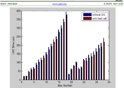
Without the injection of DG, LRIC of each node is shown in Fig.5. obviously the more downstream the node is, the higher its LRIC is, because of the longer line and higher supply cost. LRIC of bus 18 with395.22$/kw-yr and bus 17 with 352.65$/kw-yr takes the second place

,

Table 2. Economic Parameters Of DG Unit

parameters Gas

turbine Fuel cell

Wind turbine Fixed cost($/kw) 1500 3000 3000 Variable operating

Cost( $/kwh) 0.055 0.045 0.01 Subsidy,$/kwh 0 0 0.008 Life cycle,year 15 25 20 Capacity factor 1 1 0.32 Connection cost

($/kw-yr) 43.844 62.036 23.272

.

7

Fig5: Comparison Of LRIC Before And After Connection Of Fuel Cell

because of its nature. The operational and connection cost of these three types of DG units are considered as given in Table2 [9].

Now, all the buses are regarded as the candidate sites for DG, and the incremental DG capacity injected every time is chosen to be10kw[8].

The optimal locations and capacities for the three types of DG are shown in Table3. Buses 18, 19, 20, 21, 22, 23. 25, 27, 29, 31,33 appear in all three case, while bus 26 appear only in gas turbine.

Gas turbine with the capacity of 2.2MW connecting to the distribution network takes the first place. Wind turbine with the size 1.39MW takes the second place and fuel cell with the size 1.15MW takes the third place. Wind turbine has less economical efficiency than the other types of DG.

[image:7.612.89.525.68.377.2]

The variation of the total LRIC and the increase in load growth speed by an amount of 10% is shown in Fig.6. From the Fig.6 it is observed that initially for 10% of load growth speed the difference between total LRIC with DG and total LRIC without DG is high for a Gas turbine.

Table 3 Optimal DG Capacity And Location For 33 Bus System

Bus no.

DG size (kw) Gas

Turbine

Fuel cell Wind turbine

18 80 80 80

19 90 90 90

20 100 100 100

21 110 110 110

22 50 50 50

23 510 120 120

25 410 120 120

26 60 0 0

27 130 130 130

29 210 130 140

31 360 130 360

33 90 90 90

Total 2200 1150 1390

8

Fig.6 Variation Of Total LRIC Vs Load Growth Speed

turbine has lower fuel cost than others it is not. The gas turbine is most economical andefficient by forward looking than wind turbine.

6. CONCLUSIONS

This paper presents a new approach to DG sizing and siting based on LRIC and load growth control. It gives the cost details for a given DG type. .

Here DG size is established using heuristic algorithm combined with LRIC and load growth. It is not a unique solution to the problem but it is tested effectively on 33-bus distribution network. On the whole one can predict economic potential of DG connected to distribution network which is simple and cost effective

.

REFRENCES:

[1] Ferry A.Viawan, “Steady state operation and control of power distribution systems in the presence of distributed generation”, 2006. [2] Acharya N., Mahat.P., Mithulnathan N.,” An

analytical approach for DG allocation in

primary distributiom network”, Electric power and energy systems, vol.28, no.10,December 2006,pp-669-678.

[3] Rujula A.A.B., Mur Amada J., Beneral-Agustin J.L., Yusta loyo J.M., J.A, Navarro D.,”Definitions for distributed generation: a revision”, US Department of Energy 4.

[4] IEA, Electric Power Technology: Opportunities and Challenges of Competition, International Energy Agency ,France.1999.

[5] Ackermann T., Anderson G. and Soder L.,”Distributed Generation: A definition”, Electric Power System Rresearch, volume-71, pages 119-128, October 2001.

[6] Queada V.H.M., Abbad J.R., Roman T.G.S.,” Assesment of energy distribution losses for increasing penetration of distributed generation,” IEEE Transactions on power systems, Volume-21, No.2, Pages 533-540, May-2006.

9 System, Volume-22, No.4, pages.1683-1689,2007.

[8] Ouyang W., Cheng H. and Zhang X.,” Evaluation of distributed generation connecting to distribution network based on long-run incremental cost”, IET Generation, Transmission & Distribution, Vol .5, Issue-5, pages 561-568, 2011.