A DECISION-THEORETIC INTELLIGENT AGENT MODEL
YONGHUI CAO
School of Economics & Management, Henan Institute of Science and Technology
E-mail: [email protected]
ABSTRACT
Several methods are employed in multi-agent learning and organization problem such as temporal difference (TD(λ)), genetic algorithms, and learning classifier systems. The main disadvantage of these methods is that they perform badly when the data is not fully observable. In this paper, we first introduce explain learning systems in artificial intelligence(AI) and Self-organization systems. Then, we study the structure of self-organization of the intelligent agents, Finally, we design the decision-theoretic intelligent agent system, feedback control and adaptive control.
Keywords: Artificial Intelligence; Self-organization System, Decision-theoretic Intelligent, Feedback Control, Adaptive Control
1.
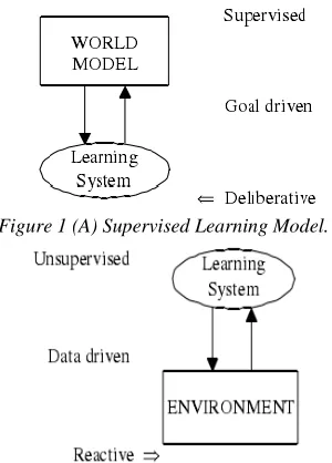
LEARNING SYSTEMS IN ARTIFICIAL INTELLIGENCEThere are two approaches to model a learning system in the AI literature. A learning system is modeled as either supervised or unsupervised. The first approach is called supervised learning in which the learning system has a world model. The learning system makes its decisions according to the world model. Some type of feedback from the environment is required to change the world model. This is also called a goal-driven learning system or a deliberative learning system. Figure 1(a) illustrates a goal driven learning system.
Figure 1 (A) Supervised Learning Model.
Figure 1 (B) Unsupervised Learning Model.
The second approach is described as supervised learning in which the learning system explores the environment and takes actions to change it. This type of learning is also called a data-driven or a reactive learning system because the learning system depends on only data, and it does not have a model of the world. Figure 1(b) illustrates an unsupervised/data-driven learning system model. There has been some research on a method that tries to combine the two learning models. The methods were combined often in ad-hoc ways and usually with limited success. This work will propose an approach that combines both types of learning models. We will call the proposed learning model the bi-directional learning model. These two approaches are used consecutively in some learning systems, but they are not usually used simultaneously.
Figure 2. Bi-Directional Learning System Model.
[image:1.612.91.241.486.695.2]2. SELF-ORGANIZATION SYSTEMS
The main idea of a self-organizing mechanism is to control a society of autonomous agents through structurization and organization. The task of adapting the structure of a group or a society of artificial agents to the environment is considered an optimization problem by characterizing a search space and an objective function to be optimized. The objective function denotes the current system's performance while a multi-dimensional search space describes the system's set of possible configurations.
The search space dimensions can be derived from principles of a multi-agent system application: structural principles, communication principles, and agent architecture principles.
Structural principles are, for example, the number of agents in the group, the number of specialists for a certain task, the organizational form of the group, migration (i.e.distribution of agents over the net), and so on. Communication principles can be expressed through the introduction of communication channels between subunits or even between agents belonging to a common subunit. Agent architecture principles are explicit resource distributions among the various agent modules. A unified approach is provided by the paper.
Self-organization of multi-agent systems is commonly achieved by using some combination of rule-based systems, Q-learning, Temporal Difference TD (λ), and evolution-based algorithms. Traditional Genetic algorithms (GAs) are well suited for off-line search, where search time is not important. Unfortunately, the domains where multi-agent systems are in use are generally highly dynamic since the environment may change anytime. In addition, a traditional GA needs to process many individuals. This might require storing the configuration of tens of complete agent societies, which is intractable. That is why the evolution-based algorithms have to be modified greatly for on-line use. Thus, the performance of a GA is inefficient in multi-agent systems.
Temporal difference and Q-learning methods are also commonly employed to solve multi-agent learning and organization problems. Temporal difference methods require learning the value function for a fixed policy. Thus, they must be combined with other reinforcement learning methods that can use the value function to make policy improvements.
Temporal difference methods work in the following way. Let V( )s denote the current
estimated value of state s under a fixed policy Π . When a sample s a t r, , , is received by performing
action α in state s at time t with the reward r, the simplest TD-method (known as TD (0)) will update the estimated value to be
(1−α)V( )s +α(r+βV( ))t
(1)
Here α is the learning rate (0≤ ≤α 1), governing to what extent the new sample replaces the current estimate. The symbol β is the discount factor. This is the basis of TD (λ), where a parameter λ captures the degree to which past states are influenced by the current sample.
Q-learning is a straightforward and elegant method for combining value function learning (as in TD-methods) with policy learning. A Q-value, Q (s a, ), is assumed for each state-action pair s a, . The Q-value provides an estimate of the value of performing action α at state s. An agent updates its estimate Q (s a, )based on sample s a t r, , , using
the formula:
}
{
(1 ) ( , ) ( (max ( , ) ))d
Q s r Q s
α α α β α′
− + + (2)
Temporal difference and Q-learning methods are successful in multi-agent learning under the assumption of full observability. Full observability means that all states of the environment can be observed completely. If the environment is not fully observable or we have incomplete data, these methods easily fail to converge. Since an agent can adopt the best policy given its current knowledge, Q-learning is only guaranteed to converge to the optimal Q-function (and implicitly an optimal policy) if each state in the environment is sampled sufficiently.
Learning classifier systems [Holland, 1986] also have been employed to solve multi-agent learning and self-organization problems. The learning classifier system (LCS) is a rule-based, message-passing, machine learning paradigm designed to process environmental stimuli, much like the input-to-output mapping provided by a neural network. The LCS provides learning through genetic and evolutionary adaptation to changing task environments. The operation of the LCS is centered around a list of rules or classifiers. These rules are essentially a set of “if-then” statements, where the “if” part of a rule is called condition, and the “then” part is called an action.
are able to generate good solutions to both a resource sharing and a robot navigation problem. They also claim that learning classifier systems can be used effectively to achieve near-optimal solutions more quickly than the Q-learning algorithm does. Even though some claim that learning classifier systems perform better than the Q-learning algorithm, these systems tend to have some deficiencies in decision-making because they are rule-based systems. Partial observability (incomplete data) is hard to handle for learning classifier systems too. Main problem with the LCS is the "bucket-brigade", which cannot converge.
Evolution-based algorithms are not efficient enough because they are not able to perform well on-line. Q-learning algorithms perform well online, but they are not able to handle the partial observability of the environment. Even though some claim that learning classifier systems perform better than Q-learning algorithms, they are not able to perform well with incomplete data. They also have some conceptual and computational difficulties to overcome.
Last, but not least, the methods described above are not completely bi-directional learning models although there is some bi-directionality in them. The importance of bi-directional learning comes from its potential to combine the supervised learning and unsupervised learning and facilitates them at the same time. The present research attempts to provide a new approach that overcomes the difficulties described above paragraphs. The new approach is based on Bayesian networks, directed acyclic graphs (DAG) that are constructed by a set of variables coupled with a set of directed edges between variables.
3. THE STRUCTURE OF AN INTELLIGENT AGENT
An agent is defined as an entity that can be viewed as perceiving environment through sensors and acting upon that environment through effectors. Therefore, an agent should have sensors and actuators to interact with the environment. On the other hand, an intelligent agent is an agent that reasons with the sensory information and creates optimal actions to satisfy a goal. Therefore, a reasoning system and a decision support system are necessary elements of an intelligent agent. Bayesian networks and influence diagrams can be considered as reasoning systems and decision support systems respectively.
Communication between the agents is also necessary to establish organizational behaviors in a multi-agent self-organizing system. Therefore, an intelligent agent should have sensors, actuators for actions, a Bayesian network, an influence diagram and a communication system.
An intelligent agent has five levels: sensors, belief, preferences, capabilities and actions. In this design, Shohams' agent oriented programming paradigm is followed. According to this paradigm, the mental state of agents can be represented in terms of their belief, capabilities, and preferences. The belief level consists of a Bayesian network (
V
A orV
E ) and its nodes represent agent's possibly uncertain beliefs about the world. The nodes inV
A represent variables related to the other agents in the system. The nodes inV
E represent the variables related to the agent itself. The preference level is represented as a utility node(
U
Aand
U
E)
that expresses the desirability of a world state. The capability level is represented by decision nodes(
V
DAand
V
DE)
that contain alternative courses of action, which the agent can execute to interact with the world. This is also called belief, desire, and intention (BDI) architecture in the literature.Each agent models other agents as an influence diagram by modeling other agents' variables
(
V
A),
utility function
(
U
A),
and decision nodes(
V
DA).
Duryadi and Gmytrasiewicz stated that other agents' models could be learned using influence diagrams. As a modeling representation tool, the influence diagram is able to express an agent's belief, capabilities and preferences, which are required if we want to predict the agent's behavior. Duryadi and Gmytrasiewicz established the learning of other agents' behaviors in the following way: Given an initial model of an agent and a history of its observed behavior, new models can be constructed by refining the parameters of the influence diagram in the initial model. The details of the learning method can be seen.
Agents also need a model of the environment. Bayesian networks can model the environment efficiently. The nodes in
V
E model the environment and provide beliefs about the environment. Then, these beliefs are dragged into the utility nodeU
E.
The utility nodeU
Eby the goal of the multi-agent organization system. The utility
U
E is a function of the belief about the environment(
V
E),
the expected actions of the other agents(
A
2),
its possibly course of actions(
A
1).
Figure 3 presents the proposed intelligent agent model.Figure3. The Structure Of An Intelligent Agent
After establishing the world model and the utility function, the agent needs to take an optimal action according to the principle of maximum expected utility (PMEU). The PMEU lets the agents choose the best action from its set of action
(
A
1),
given the belief about the environment(
V
E), a
nd other agents' expected behavior(
A
2).
Formally, it can be expressed as{
}
1
1 2
max
max
,
,
i
E E
a
U
=
f V
A A
(3)
Where
V
E=
{
X
1,
X
2,
,
X
n}
,
the variablesi
X
are the nodes of the Bayesian networkV
E,
{
}
1 11
,
12,
,
1kA
=
a
a
a
is the action set of the agent,A
2=
{
a
21,
a
22,
,
a
2i}
is the expected action set of the other agents. Therefore, an agent takes its actions after evaluating the environment and the other agents. This property will help to obtain self-organization ability of the system. Each agent first check to see if other agents areperforming task before it takes its actions to perform the task.
4. MULTI-AGENT SELF-ORGANIZING SYSTEM SCHEME
This section will examine the learning problem when we have more than one agent. The agent described in the previous section is specifically designed for multi-agent systems. In a multi-agent environment, coordination requires an agent to recognize the current status and to model the actions of the other agents to decide on its own next
behavior. That's why agents model other agents as well as the environment. A computational difficulty may arise if the number of agents is large in the system because agents model the internal structure of other agents in their network. The Bayesian network in the agent may become so large that the calculation of the conditional probabilities might become difficult. The agents are independent but they take their actions by considering the other agents. Thus, agents take their actions together in coordination. Formally speaking, the agent's utility function
U
E depends on the expected actions of other agents (A
1), see Equation (3).We can explain this ability with an example. Suppose we have two dogs and a sheep, as in the sheepdog problem. Dogs are our agents and their goal is to put the sheep into a barn. Dogs will explore the environment and they will model the environment. In this case, the environment contains another dog, a sheep, and a barn. First, the dogs will probably locate the sheep. Then, they will make movements to direct the sheep into the barn. If the dogs do not consider (model) each other, they might not be able to put the sheep into the barn since one's action might hinder the other's action. Thus, they need to cooperate and make movements together. If each dog learns the model of the other dog, then they can make movements together to put the sheep into the barn. If there is no coordination, both dogs will probably go behind the sheep and direct it into the barn. If there is coordination between the dogs, while one of them goes behind the sheep, the other may move back and forth so that the sheep will not escape as shown in Figure 4.
Figure4. Multi -Agent Behavior Without Coordination (A) And With Coordination (B)
A multi-agent self-organization system with two agents can be seen in Figure 5. The multi-agent system is designed by using the agents, shown in Figure 3.
Self-organization will happen eventually because each agent takes its actions considering other agents' behaviors in the environment. This property will make our system a multi-agent self-organizing system. In the proposed learning system, an agent learns the environment using the sensory data, and modifying its world model (Bayesian Network) accordingly. Then, an agent calculates the expected state of the environment using the world model and creates actions to change the environment. Thus, the learning structure is bi-directional because the agent interacts with nature and the world model in both directions.
Figure5. Multi-Agent Self-Organizing Scheme With Two Agents
5. THE DECISION-THEORETIC INTELLIGENT SYSTEM
The decision-theoretic intelligent agent system has adaptive learning ability with feedback from the environment. The agent starts with a limited knowledge of the plant (environment), then it explores (samples) the plant to learn the plant's parameters. After it learns about the plant, it takes its actions accordingly. The agent first estimates the plant's behavior using the previous observation, and then takes its action according to the estimation. The plant, then responds to the agent's action with an output. The output of the plant in this stage is used as feedback to update the plant parameters in the predictor (BN). Figure 6 shows the decision theoretic-intelligent agent learning system in a block diagram.
In Figure 6,
I X
( )
represents the initial state of the plant,E X
( )
ˆ
is the expected value of the state,( )
E y
is the expected value of the plant output,and
y
GOAL is the desired plant (system) output. The symbolq
−1 represents one unit delay. The controller (ID) applies controls to the plant to provide a certain plant output because the controller creates the control according to the error between the expected value of the plant output and the reference. The reference is the desired output to be provided by the plant. The observer (BN) models the plant by using the plant's input/outputs. After a control is applied to the plant, the plant output is used in the next step to update the plant model. Thus, there is a time delay between the control and the output of the plant. The controller creates the control using a priori knowledge about the plant (environment).Figure6. System Block Representation Of The Intelligent Agent System
The decision theoretic intelligent agent system (DTAS) has potential use in feedback control and adaptive control because it uses the plant's output as a feedback and modifies the controller and the observer accordingly.
5.1 Feedback Control
In the literature, there are two main types of feedback control, namely output feedback and state feedback. Output feedback is performed by a path (loop) from the output back to the controller as shown in Figure 7.
Figure7. Output Feedback Control
The equations for the system in Figure 6 can be given as:
ˆ
GOAL( )
u
=
f e
(5)( )
y
=
g u
(6)Now, let us compare the system equations in the
feedback control system and the decision-theoretic
intelligent agent system. In the DTAS, the output of
the plant,
y
, also depends on the control input,u
. Let us compare the control signalu
in both systems.( )
( )
DTAS FEEDBACK
u
=
h e
⇔
u
=
f e
(7)If we choose the functions
h
andf
to be equal, then the controllers will give the same controlu
with the same error
e
. Let us compare the errors in both systems. In the DTAS, the error is the difference between the desired output and the expected value of the plant output provided by the predictor. This is very similar to the feedback control system but the expected value of the plant output replaces the measured plant output. These two values are equivalent only if the predictor estimates the output of the plant well enough. In the DTAS, it is shown that the predictor estimates the plant output well enough when there is sufficient data from the plant's input/output. Therefore, the expected value in the DTAS is equivalent to the measured value of the plant output in a feedback control system. The following equations summarize the discussion.( )
GOALe
=
y
−
E y
(8)ˆ
( )
E y
≅
y
(9)ˆ
GOALe
=
y
−
y
(10)From Equations (8), (9), and (10), we may conclude that the DTAS exhibits feedback control properties.
Another type of feedback control is state feedback control. In state feedback control, the state variables are sensed and fed back to the input through appropriate gains. If there is direct access to the state variables, the state variables can be easily measured and fed back to the input. If there is no direct access to the state variables, then an observer may be employed to perform the estimation of the state variables. Figure 8 illustrates a state feedback control system with an observer.
The block denoted by
FE
is the plant. The estimator predicts the state variables of the plant. The estimated state variables are fed to the input with a gainK
. Then, the control signal becomes the following:ˆ
u
= +
r
KX
(11)Figure8. A Control System With The State Feedback
Thus, the control is a function of estimated state variables and the reference input. Let us compare the controls in both systems. In the DTAS, the control is defined as
( )
u
=
f e
(12)where
e
=
y
GOAL−
y
ˆ
.The termy
ˆ
represents the estimated output of the plant. The termy
ˆ
is a function of the estimated state variables because itis calculated by the utility function of the system.
Therefore, we can represent
y
ˆ
with the following equation.ˆ ˆ
ˆ
y
=
CX
(13)where the vector
X
ˆ
is the estimated state vector and the matrixC
ˆ
is the transformation matrix between the states and the output. Thus, the controlcan be rewritten as follows:
ˆ
(
GOAL)
u
=
f y
−
y
(14)ˆ ˆ
( )
(
GOAL)
u X
=
f y
−
CX
(15) Let us assume that the function f is a linearfunction with the following form.
( )
f x
= ⋅
A x
(16)ˆ
ˆ
ˆ
ˆ
(
GOAL)
GOALu
= ⋅
A
y
−
CX
= ⋅
A y
− ⋅
A CX
(17)Let
K
= − ⋅
A C
ˆ
,andr
= ⋅
A y
GOAL, then thecontrol becomes
ˆ
u
= + ⋅
r
K X
(18)As seen in Equation (18), the control signal in
the DTAS can be interpreted as the control signal in
the state feedback control. This concludes the
analysis of how the DTAS corresponds to a
feedback control system. It can be concluded that
the DTAS will have the inherent advantages of
feedback control. The following section
investigates the adaptive control capabilities of the
5.2 Adaptive Control
The term adaptive control covers a set of methods that provide a systematic approach for automatic adjustment of the controllers in real time, in order to achieve or to maintain a desired level of performance of the control system when the parameters of the plant dynamic model are unknown and/or change in time. A block diagram presenting a basic configuration of an adaptive control system is shown in Figure9.
Figure9. A Basic Adaptive Control System
The following definition provides an adaptive control system given in Figure 6. An adaptive control system calculates a certain performance index (IP) of the control system using the measured inputs, the states, the outputs, and the known disturbances. From the comparison of the performance index and a set of given ones, the adaptation mechanism modifies the parameters of the adjustable controller and/or generates an auxiliary control signal in order to maintain the performance index of the control system close to the set of given ones (i.e., within the set of acceptable ones).
An adaptive control system will monitor the performance of the system in the presence of parameter disturbances in addition to a feedback controller with adjustable parameters acting as a supplementary loop upon the adjustable parameters of the controller.
There are three types of adaptive control schemes in the literature: open loop adaptive control, direct adaptive control, and indirect adaptive control. In open loop adaptive control, the adaptation mechanism is a simple look-up table stored in the computer that gives the controller parameters for a
given set of environment measurements. In the literature, this is also called gain-scheduling.
Direct adaptive control is based on the observation that the difference between the output of the plant and the output of the reference model (called plant-model error) is a measure of the difference between the real and the desired performance. The reference model is a realization of the system with desired performance. This information is used by the adaptation mechanism (called parameter adaptation) to directly adjust the parameters of the controller in real-time in order to force (asymptotically) the plant model-error to zero. This scheme corresponds to the use of Model Reference Adaptive Systems (MRAS) for the purpose of a general concept called Model Reference Adaptive System (MRAS) for the purpose of control. The indirect adaptive control was originally introduced by Kalman.
In an indirect adaptive control system, shown in Figure 10, the basic idea is that a suitable controller can be designed on line if a model of the plant is estimated on line from the available input-output measurements. The scheme is called indirect because the adaptation of the controller parameters is performed in two stages:
1 .On-line estimation of the plant parameters (e.g. Bayesian network construction)
2. On-line computation of the controller parameters based on the current estimated plant model (e.g. Influence Diagrams-making decisions)
Figure10. Indirect Adaptive Control System
sampling instant will adjust the parameters of the adjustable predictor in order to minimize the prediction error in the sense of a certain criterion.
There are two options given to effectively implement an indirect adaptive control strategy. The choice is related to a certain extent to the ratio between the computation time and the sampling period.
Strategy 1:①Sample the plant output;②Update the plant model parameters; ③ Compute the controller parameters based on the new plant model parameter estimates;④Compute the control signal; ⑤Apply the control signal;⑥Wait for the next sample.
In this strategy, there is a delay between
u t
( )
and
y t
( )
. This delay should be smaller than the sampling period.Strategy 2:①Sample the plant output;②Compute the control signal based on the controller parameters computed during the previous sampling periods;③Apply the control signal;④Update the plant model parameters;⑤Compute the controller parameters based on the new plant model parameter estimates;⑥Wait for the next sample.
In the second strategy, the delay between
u t
( )
and
y t
( )
is smaller than in the previous case. In this strategy, a priori parameter estimation is performed since we apply the control without updating the plant parameters.In the above paragraphs, a general definition of an adaptive control system is provided. A greater importance is given to indirect adaptive control systems because the decision-theoretic agent system (DTAS) has the properties of an indirect adaptive control system. The DTAS has the same steps as the indirect adaptive control system. Additionally, the learning strategy in DTAS is very similar to the second strategy of the indirect adaptive control system.
The first step, the on-line estimation of the plant model parameters, is performed by structuring a Bayesian network and calculating its parameters in the DTAS. The online Bayesian network learning is performed to model the plant. The second step, the online computation of the controller parameters, is performed by a decision system (influence diagrams).
As shown in Figure 5, there are two adaptation mechanisms in the indirect adaptive control. The
first adaptation mechanism corresponds to the online Bayesian network learning in the DTAS. The second adaptation mechanism corresponds to the utility node in the influence diagram part of the decision-theoretic intelligent agent because it determines which action will be fired in the decision node. The adjustable predictor corresponds to the Bayesian network in the DTAS. Finally, the adjustable controller corresponds to the decision nodes in the influence diagram in the DTAS.
Now, the indirect adaptive control system can be redrawn by using the decision-theoretic intelligent agent components, shown in Figure11.
Figure11. Indirect Adaptive Control Representation Of The DTAS
Consequently, the online Bayesian learning determines the plant model structure and parameter estimation; and, the influence diagram determines the controller parameters. Therefore, it can be concluded that the decision-theoretic intelligent agent system implements an indirect adaptive control system.
6 . CONCLUSIONS
environment. The agent starts with a limited knowledge of the plant (environment), then it explores (samples) the plant to learn the plant's parameters. After it learns about the plant, it takes its actions accordingly.
REFRENCES:
[1] C. Gerber, "Evolution-based self-adaption as an expression for the autonomy degree in multi-agent societies," in Proceedings of the IEEE Joint Conference on the Science and Technology of Intelligent Systems, Gaithersburg, MD, pp. 741-746, September 1998.
[2] D. Suryadi and P. J. Gmytrasiewicz, "Learning models of other agents using influence diagrams," in Proceedings of User Modeling: The Seventh International Conference, Springer Wien, New York, 1999, to apper.
[3] J. Pearl, "Constraint-propagation approach to probabilistic reasoning," in L. M. Kanal and J. Lemmer (Eds.), Uncertainty in Artificial Intelligence, North-Holland, Amsterdam, pp. 357-288, 1986.
[4] J. Pearl, Probabilistic Reasohihg in Intelligent Systems: Networks of Plausible Inference. San Mateo, CA: Morgan Kaufmann, 1988.
[5] J. Pearl, "A probabilistic calculus of actions," in Proceedings of the Tenth Conference oh Uncertainty in AI (UAI-94), San Mateo, CA: Morgan Kaufmann, 1994.
[6] N. Friedman, K. Murphy, and S. Russell, "Learning the structure of dynamic probabilistic networks," in G.F. Cooper and S. Moral (Eds.), Proceedings of Fourteenth Conference oh Uncertainty in Artificial Intelligence (UAI '98), San Francisco, CA: Morgan Kaufmann, 1998. [7] S. L. Lauritzen and D. J. Spiegelhalter, "Local
computations with probabilities on graphical structures and their application to expert systems," Journal of the Royal Statistical Society, Series B, vol. 50(2), pp. 157-224, 1988.
[8] S. Non and P. J. Gmytrasiewic, "Coordination and belief update in a distributed anti-air environment," in Proceedings of the 31S' Hawaii International Conference on System Sciences, vol. V, pp. 142-145, Los Alamitos, CA: IEEE Computer Society, January 1998. [9] S. Sen and M. Sekaran, "Multi-agent
coordination with learning classifier systems," in Proceedings of the IJCAI Workshop oh Adaptation and Learning in Multi-agent Systems, Montreal, pp. 84-89, 1995.
[10] S. Russell and P. Norvig, Artificial Intelligence: A modern Approach, New Jersey: Prentice Hall, 1995.
[11] T. Malsch and I. Schulz-Schafer, "Generalized media of interaction and inter-agent coordination," in Socially Intelligent Agents-Papers from the 1997 AAAI Fall Symposium, Technical Report FS-97-02, AAAI, 1997. [12] Y. Shoham, Agent-oriented programming,"