R E S E A R C H
Open Access
Gradient projection method with a new
step size for the split feasibility problem
Pattanapong Tianchai
1**Correspondence:
1Faculty of Science, Maejo
University, Chiangmai, Thailand
Abstract
In this paper, we introduce an iterative scheme using the gradient projection method with a new step size, which is not depend on the related matrix inverses and the largest eigenvalue (or the spectral radius of the self-adjoint operator) of the related matrix, based on Moudafi’s viscosity approximation method for solving thesplit feasibility problem(SFP), which is to find a point in a given closed convex subset of a real Hilbert space such that its image under a bounded linear operator belongs to a given closed convex subset of another real Hilbert space. We suggest and analyze this iterative scheme under some appropriate conditions imposed on the parameters such that another strong convergence theorems for the SFP are obtained. The results presented in this paper improve and extend the main results of Tian and Zhang (J. Inequal. Appl. 2017:Article ID 13, 2017), and Tang et al. (Acta Math. Sci.
36B(2):602–613, 2016) (in a single-step regularized method) with a new step size, and many others. The examples of the proposed SFP are also shown through numerical results.
MSC: 47H05; 47H09; 47H20
Keywords: Split feasibility problem; Split common fixed point problem; Gradient projection method
1 Introduction
Throughout this paper, we always assume thatCandQbe closed convex subsets of two real Hilbert spacesHandK, respectively with inner product and norm are denoted by·,· and · , respectively. LetA:H→K be a bounded linear operator. Thesplit feasibility problem(SFP) which was first introduced by Censor and Elfving [3] is to find
x∗∈C such that Ax∗∈Q. (1.1)
Suppose thatPCandPQare the orthogonal projections onto the setsCandQ, respectively. Assume that SFP (1.1) is consistent. We observe thatx∗∈Csolves the SFP (1.1) if and only if it solves the fixed point equation
x∗=PC
I–γA∗(I–PQ)A
x∗,
whereγ > 0 is any positive constant,Iis the identity operator onHorK, andA∗denotes the adjoint ofA. To solve SFP (1.1) in the setting of a finite-dimensional real Hilbert space
case, Byrne [4] proposed the so-calledCQalgorithm based on the Picard iteration method as follows:
xn+1=PC
I–γAt(I–PQ)A
xn, ∀n= 0, 1, 2, . . . , (1.2)
whereγ∈(0,2L) such thatLbeing the largest eigenvalue of the matrixAtAasAtstands for matrix transposition ofA. He proved that the sequence{xn}generated by (1.2) converges strongly to the SFP (1.1).
In [5], Yang presented a relaxedCQalgorithm for solving the SFP (1.1), where he used two halfspacesCnandQnin place ofCandQ, respectively, and at thenth iteration, the orthogonal projections ontoCnandQnare easily executed.
Both theCQalgorithm and the relaxedCQalgorithm used a fixed step size related to the largest eigenvalue of the matrixA∗Aor the spectral radius of the self-adjoint operator
A∗A, which sometimes affects convergence of the algorithms. In [6], Qu and Xiu presented a modification of theCQalgorithm and the relaxedCQalgorithm by adopting the Armijo-like searches, which need not to compute the matrix inverses and the largest eigenvalue of the matrixA∗A. TheCQ-like algorithms are also proposed subsequently [3, 7–10].
In all theseCQ-like algorithms for the SFP (1.1), in order to get the step size, one has to compute the largest eigenvalue of the related matrix or use some line search scheme which usually requires many inner iterations to search for a suitable step size in every iteration. We note that a pointxsolves the SFP (1.1) means that there is an elementx∈Csuch that Ax–x∗= 0 for somex∗∈Q. This motivates us to consider the distance function
d(Ax,x∗) =Ax–x∗for allx∈C, and the constrained convex minimization problem:
min
x∈C,x∗∈Q 1 2Ax–x
∗2
such that minimizing with respect tox∗∈Q. Letg:C→Rbe a continuous differentiable function. First makes us consider the minimization:
min
x∈Cg(x) := 1
2Ax–PQAx
2 (1.3)
is ill-posed. Therefore, Xu [11] considered the following Tikhonov regularization problem:
min
x∈Cg(x) :=g(x) + 2x
2=1
2Ax–PQAx
2+
2x
2,
where> 0 is the regularization parameter. We know that the gradient∇gofgas
∇g(x) =∇g(x) +I=A∗(I–PQ)A+I, ∀x∈C,
such that ∇g(x) is ( +A2)-Lipschitzian continuous (that is, ∇g(x) –∇g(y) ≤ (+A2)x–yfor allx,y∈C) and-strongly monotone (that is,∇g
(x) –∇g(y),x–y ≥
x–y2for allx,y∈C).
the setting of an infinite-dimensional real Hilbert space as follows:
xn+1=PC(I–γn∇gn)xn =PC
I–γn
A∗(I–PQ)A+nI
xn, ∀n= 0, 1, 2, . . . . (1.4)
He proved that the sequence{xn}generated by (1.4) converges in norm to the minimum-norm solution (1.3) of the SFP (1.1), provided the parameters{n},{γn} ⊂(0, 1) satisfy the following conditions:
(i) limn→∞n= 0and0 <γn≤A2n+
n, (ii) ∞n=0nγn=∞,
(iii) limn→∞|γn+1–(γn|+γn|n+1–n| n+1γn+1)2 = 0.
In [1], Tian and Zhang suggested a single-step regularized method based on the Picard iteration method in the setting of an infinite-dimensional real Hilbert space as follows:
xn+1=PC(I–λ∇gn)xn =PC
I–λA∗(I–PQ)A+nI
xn, ∀n= 0, 1, 2, . . . . (1.5)
They proved that the sequence{xn}generated by (1.5) converges in norm to the minimum-norm solution (1.3) of the SFP (1.1), provided the parameters{n} ⊂(0, 1) andλsatisfy the following conditions:
(i) 0 <λ< 2
A2+2,
(ii) limn→∞n= 0and∞n=0n=∞, (iii) ∞n=0|n+1–n|<∞.
We observe that in the proof of their proposed results,∞n=0|n+1–n|<∞of the control
condition (iii) can be removed using the NST-condition (II) [12] (see also [13, 14]). The SFP (1.1) is an important and has been widely studied because it plays a prominent role in the signal processing and image reconstruction problem. Initiated by the SFP, sev-eral split type problems have been investigated and studied, for examples, the split vari-ational inequality problem (SVIP) (see [15]) and the split common null point problem (SCNP). We will consolidate these problems. LetS:H→HandT:K→Kbe two oper-ators with nonempty fixed point setsFix(S) :={x∈H:x=S(x)}andFix(T), respectively. IfSbe a nonexpansive mapping (that is,Sx–Sy ≤ x–yfor allx,y∈H), thenFix(S) is closed and convex (see [16]). Thesplit common fixed point problem(SCFP) is to find
x∗∈Fix(S) such that Ax∗∈Fix(T). (1.6)
IfS=PCandT=PQthenFix(S) =CandFix(T) =Q, and hence the SCFP (1.6) immedi-ately reduces to the SFP (1.1).
Assume that the SCFP (1.6) is consistent. In [17], Censor and Segal proposed and proved a strong convergence theorem for the SCFP (1.6) based on the Picard iteration method, in the case that the directed operatorsS(that is,x–Sx,Sx–y ≥0 for ally∈Fix(S) and
x∈H, for instanceS=PC) andT, still in a finite-dimensional real Hilbert space to extend the iteration method (1.2) of Byrne as follows:
xn+1=S
I–γAt(I–T)Axn, ∀n= 0, 1, 2, . . . ,
In [18], Kraikaew and Saejung proposed and proved a strong convergence theorem for the SCFP (1.6) based on the Halpern iteration method, in the case that the quasi-nonexpansive mappingsS (that is,Sx–p ≤ x–pfor allx∈Handp∈Fix(S)) and
T such that bothI–SandI–T are demiclosed at zero on an infinite-dimensional real Hilbert space as follows:
xn+1=αnx0+ (1 –αn)S
I–γA∗(I–T)Axn, ∀n= 0, 1, 2, . . . ,
whereγ ∈(0,1
L),{αn} ⊂(0, 1),limn→∞αn= 0 and
∞
n=0αn=∞.
In [2], Tang et al. proposed and proved a strong convergence theorem for the SCFP (1.6) based on the viscosity approximation method, in the case that the firmly nonexpansive mappingsS(that is,Sx–Sy2≤ x–y2–(I–S)x– (I–S)y2for allx,y∈H) andTsuch
that bothI–SandI–Tare demiclosed at zero, and anα-contraction mappingh:H→H
withα∈(0, 1) (that is,h(x) –h(y) ≤αx–yfor allx,y∈H) on an infinite-dimensional real Hilbert space in a single-step regularized method as follows:
xn+1=αnxn+βnh(xn) +γnS
I–ξnA∗(I–T)A
xn, ∀n= 0, 1, 2, . . . ,
whereαn+βn+γn= 1,ξn= ρn(I–T)Axn
2
2A∗(I–T)Axn2,{ρn} ⊂(0, 4),{αn},{βn},{γn} ⊂(0, 1) satisfy the
following conditions: (i) limn→∞βn= 0and
∞
n=0βn=∞, (ii) lim infn→∞αnγn> 0.
We observe that in the proof of their proposed results, the sequence{ξn}may not con-verges to the zero, for instance ifA=Iandρn= 2 for alln= 0, 1, 2, . . . then the sequence {ξn}converges to the integer 1. The relaxedCQ-like algorithms are also proposed subse-quently [19–21].
In this paper, we modify in all these algorithms to solve the SCFP (1.6) and also solve the SFP (1.1) based on Moudafi’s viscosity approximation method [22], in the case that the firmly nonexpansive mappingsSandT such that bothI–SandI–Tare demiclosed at zero, and anα-contraction mappingh:H→Hwithα∈(0, 1) on an infinite-dimensional real Hilbert space in a single-step regularized method with the regularization parameter as follows:
xn+1=αnxn+βnh(xn) +γnS
I–λn
A∗(I–T)A+nI
xn, ∀n= 0, 1, 2, . . . . (1.7)
We suggest and analyze this iterative scheme (1.7) under some appropriate conditions imposed on the parameters with a new step size, which is not depend on the related matrix inverses and the largest eigenvalue (or the spectral radius of the self-adjoint operator) of the related matrix such that another strong convergence theorems for the SCFP (1.6) and the SFP (1.1) are obtained.
2 Preliminaries
LetH andK be two real Hilbert spaces,A:H→K be a bounded linear operator, A∗
the notation:→to denote the strong convergency, to denote the weak convergency,
ωw(xn) =
x:∃{xnk} ⊂ {xn}such thatxnk x
to denote the weak limit set of{xn}andFix(T) ={x:x=Tx}to denote the fixed point set of the mappingT.
LetC be a nonempty closed convex subset of a real Hilbert spaceH. Recall that the metric projection PC:H→C is defined as follows: for eachx∈H, PCxis the unique point inCsatisfying
x–PCx=inf
x–y:y∈C.
Letf :H→Rbe a function. Recall that a functionf is called convex if
fλx+ (1 –λ)y≤λf(x) + (1 –λ)f(y), ∀λ∈[0, 1],∀x,y∈H.
A differentiable functionf is convex if and only if for eachx∈H, we have the inequality:
f(z)≥f(x) +∇f(x),z–x, ∀z∈H.
An elementg∈His said to be a subgradient off atx∈Hif we have the subdifferentiable inequality
f(z)≥f(x) +g,z–x, ∀z∈H.
A functionf is said to be subdifferentiable atx∈H, if it has at least one subgradient atx. The set of subgradients off atx∈His called the subdifferentiable off atx, and it is de-noted by∂f(x). A functionf is called subdifferentiable, if it is subdifferentiable at allx∈H. If a functionf is differentiable and convex, then its gradient and subgradient coincide. A functionf is called lower semi-continuous (lsc) for allx∈Hif for eacha∈R, the set {x∈H:f(x)≤a}is a closed set, and a functionf is called weakly lower semi-continuous (w-lsc) atx∈Hiff is lsc atxfor a sequence{xn} ⊂Hsuch thatxn x.
We collect some known lemmas and definitions which are our main tools in proving the our results.
Lemma 2.1 Let H be a real Hilbert space.Then,for all x,y∈H,
(i) x+y2=x2+ 2x,y+y2, (ii) x+y2≤ x2+ 2y,x+y.
Lemma 2.2 ([23]) Let C be a nonempty closed convex subset of a real Hilbert space H.
Then:
(i) z=PCx⇔ x–z,z–y ≥0,∀x∈H,y∈C,
(ii) z=PCx⇔ x–z2≤ x–y2–y–z2,∀x∈H,y∈C, (iii) PCx–PCy2≤ x–y,PCx–PCy,∀x,y∈H.
(i) monotone if
x–y,Tx–Ty ≥0, ∀x,y∈H,
(ii) L-Lipschitzian withL> 0if
Tx–Ty ≤Lx–y, ∀x,y∈H,
(iii) α-contraction if it isα-Lipschitzian withα∈(0, 1), (iv) nonexpansive if it is1-Lipschitzian,
(v) firmly nonexpansive if
Tx–Ty2≤ x–y2–(I–T)x– (I–T)y2, ∀x,y∈H.
Lemma 2.4([24]) Let H and K be two real Hilbert spaces and let T:K→K be a firmly nonexpansive mapping such that(I–T)xis a convex function from K toR= [–∞, +∞].
Let A:H→K be a bounded linear operator and f(x) =12(I–T)Ax2for all x∈H.Then: (i) ∇f(x) =A∗(I–T)Ax,∀x∈H,
(ii) ∇f isA2-Lipschitzian.
Lemma 2.5([24]) Let H be a real Hilbert space and T:H→H be an operator.The fol-lowing statements are equivalent:
(i) Tis firmly nonexpansive,
(ii) Tx–Ty2≤ x–y,Tx–Ty,∀x,y∈H,
(iii) I–Tis firmly nonexpansive.
Lemma 2.6([25]) Let H be a real Hilbert space and let{xn}be a sequence in H.Then,for any given sequence{λn}∞n=1⊂(0, 1)with∞n=1λn= 1and for any positive integer i,j with
i<j,
∞
i=1
λnxn
2
≤
∞
i=1
λnxn2–λiλjxi–xj2.
Lemma 2.7([26]) Let{an}be a sequence of nonnegative real numbers such that
an+1≤(1 –γn)an+γnσn, ∀n= 0, 1, 2, . . . ,
where{γn}is a sequence in(0, 1)and{σn}is a sequence inRsuch that
(i) ∞n=0γn=∞, (ii) lim supn→∞σn≤0or
∞
n=0|γnσn|<∞.
Thenlimn→∞an= 0.
Lemma 2.8([27]) Let{tn}be a sequence of real numbers such that there exists a subse-quence{ni}of{n}such that tni<tni+1 for all i∈N.Then there exists a nondecreasing
se-quence{τ(n)} ⊂Nsuch thatτ(n)→ ∞,and the following properties are satisfied by all
(sufficiently large)numbers n∈N:
In fact,
τ(n) =max{k≤n:tk<tk+1}.
Lemma 2.9([28] (Demiclosedness principle)) Let C be a nonempty closed convex subset of a real Hilbert space H and let S:C→C be a nonexpansive mapping withFix(S)=∅.If the sequence{xn} ⊂C converges weakly to x and the sequence{(I–S)xn}converges strongly to y.Then(I–S)x=y;in particular,if y= 0then x∈Fix(S).
Lemma 2.10([16]) Let C be a nonempty closed convex subset of a Hilbert space H and let f be a proper convex lower semi-continuous function of C into(–∞,∞].If{xn} be a bounded sequence of C such that xn x0.Then f(x0)≤lim infn→∞f(xn).
3 Main result
Throughout this paper, we let:={x∈Fix(S) :Ax∈Fix(T)}. It is clear thatis closed and convex.
Theorem 3.1 Let H and K be two real Hilbert spaces and let S:H→H and T:K→K be two firmly nonexpansive mappings such that both I–S and I–T are demiclosed at zero.Let(I–T)xbe a convex function from K toRand A:H→K be a bounded linear operator,and let h:H→H be anα-contraction mapping.Assume that the SCFP(1.6)has a nonempty solution setand let{xn} ⊂H be a sequence generated by
⎧ ⎨ ⎩
x0∈H,
xn+1=αnxn+βnh(xn) +γnS(xn–λn∇gn(xn)), ∀n= 0, 1, 2, . . . ,
whereαn+βn+γn= 1and gn(xn) = 21(I–T)Axn2+2nxn2such that
∇gn(xn) =A∗(I–T)Axn+nxn= 0, λn=
ρngn(xn)
∇gn(xn)2+∇gn(xn)+ρngn(xn)
for all n= 0, 1, 2, . . . .If the sequences{ρn} ⊂[a,b]for some a,b∈(0, 2),{αn} ⊂[c,d]for some c,d∈(0, 1)and{βn},{γn} ⊂(0, 1)satisfy the following conditions:
(i) 0≤n≤βn2msuch thatm> 1for alln= 0, 1, 2, . . .,
(ii) limn→∞βn= 0and
∞
n=0βn=∞,
then the sequence{xn}converges strongly to x∗∈where x∗=Ph(x∗).
Proof Fixn∈N∪ {0}. Note thatgn(x) =12(I–T)Ax2+
n
2x
2is Gáteaux differentiable
by the convexity of(I–T)Axfor allx∈H. First, we show that{xn}is bounded. Pick
p∈. We havep∈Fix(S) andAp∈Fix(T). Observing thatI–Tis firmly nonexpansive, by Lemma 2.5 we have
xn–p,∇gn(xn) =
xn–p,A∗(I–T)Axn+nxn
=xn–p,A∗(I–T)Axn +nxn–p,xn
+n 2
xn–p2+xn2–p2
≥(I–T)Axn– (I–T)Ap
2
+n 2
xn2–p2
≥1
2(I–T)Axn
2
+n 2
xn2–p2
≥gn(xn) – β2m
n 2 p
2. (3.1)
Therefore, by the nonexpansiveness ofSwe have
Sxn–λn∇gn(xn)
–p2
=Sxn–λn∇gn(xn)
–Sp2
≤xn–λn∇gn(xn) –p
2
=xn–p2+λn2∇gn(xn)
2
– 2λn
xn–p,∇gn(xn)
≤ xn–p2+λn2∇gn(xn)
2
– 2λngn(xn) +λnβn2mp2 ≤ xn–p2+
ρn2g2
n(xn)(∇gn(xn)2+∇gn(xn)+ρngn(xn)) (∇gn(xn)2+∇gn(xn)+ρngn(xn))2
– 2ρng
2
n(xn)
∇gn(xn)2+∇gn(xn)+ρngn(xn)
+βn2mp2
=xn–p2–ρn(2 –ρn)
g2
n(xn)
∇gn(xn)2+∇gn(xn)+ρngn(xn)
+βn2mp2
≤ xn–p2+βn2mp2 ≤xn–p+βnmp
2
. (3.2)
This implies that
Sxn–λn∇gn(xn)
–p≤ xn–p+βnmp. (3.3)
Hence,
xn+1–p=αnxn+βnh(xn) +γnS
xn–λn∇gn(xn)
–p
≤αnxn–p+βnh(xn) –p+γnS
xn–λn∇gn(xn)
–p
≤αnxn–p+βnh(xn) –h(p)+βnh(p) –p
+γn
xn–p+βnmp
≤αnxn–p+βnαxn–p+βnh(p) –p+γnxn–p+βnp
=1 – (1 –α)βn
xn–p+ (1 –α)βn
h(p) –p+p
1 –α
≤max
xn–p,
h(p) –p+p
1 –α
By induction, we have
xn–p ≤max
x0–p,
h(p) –p+p
1 –α
.
This implies that{xn}is bounded, and so are{h(xn)}and{gn(xn)}. Using Lemma 2.6 and (3.2), we have
xn+1–p2=αnxn+βnh(xn) +γnS
xn–λn∇gn(xn)
–p2
=αn(xn–p) +βn
h(xn) –p
+γn
Sxn–λn∇gn(xn)
–p2
≤αnxn–p2+βnh(xn) –p
2
+γnS
xn–λn∇gn(xn)
–p2
–αnγnS
xn–λn∇gn(xn)
–xn
2
≤αnxn–p2+βnh(xn) –p
2
+γn
xn–p2
–ρn(2 –ρn) g
2
n(xn)
∇gn(xn)2+∇gn(xn)+ρngn(xn)
+βn2mp2
–αnγnS
xn–λn∇gn(xn)
–xn2 ≤ xn–p2+βnh(xn) –p
2
–γnρn(2 –ρn) g
2
n(xn)
∇gn(xn)2+∇gn(xn)+ρngn(xn)
+βnp2
–αnγnS
xn–λn∇gn(xn)
–xn2. Therefore,
γnρn(2 –ρn)
g2
n(xn)
∇gn(xn)2+∇gn(xn)+ρngn(xn) +αnγnS
xn–λn∇gn(xn)
–xn
2
≤ xn–p2–xn+1–p2+βnh(xn) –p
2
+βnp2. (3.4)
SincePhis a contraction onH, by the Banach contraction principle there exists a unique elementx∗∈Hsuch that x∗=Ph(x∗). That isx∗∈. Now, we show thatxn→x∗ as
n→ ∞. We consider into two cases.
Case 1. Assume that{xn–p}is a monotone sequence. In other words, for n0large
enough,{xn–p}n≥n0is either nondecreasing or nonincreasing. As{xn–p}is bounded,
so{xn–p}is convergent. Therefore, by (3.4) we have
lim
n→∞γnρn(2 –ρn)
g2
n(xn)
∇gn(xn)2+∇gn(xn)+ρngn(xn)
= 0 (3.5)
and
lim
n→∞αnγnS
xn–λn∇gn(xn)
–xn
2
By Lemma 2.4, we have
∇gn(xn)≤∇gn(xn) –∇gn(p)+∇gn(p)
≤A∗(I–T)Axn–A∗(I–T)Ap+nxn–p+∇gn(p) ≤A2+n
xn–p+∇gn(p) ≤A2+ 1xn–p+∇gn(p).
This implies that{∇gn(xn)}is bounded, and so is{∇gn(xn)2+∇gn(xn)+ρngn(xn)}. Hence,∇gn(xn)2+∇gn(xn)+ρngn(xn) <δfor someδ> 0. Since
(1 –d–βn)a(2 –b)
g2
n(xn) δ
≤γnρn(2 –ρn)
g2
n(xn)
∇gn(xn)2+∇gn(xn)+ρngn(xn) ,
by (3.5) we have
lim
n→∞gn(xn) = 0. (3.7)
Since
c(1 –d–βn)S
xn–λn∇gn(xn)
–xn
2
≤αnγnS
xn–λn∇gn(xn)
–xn
2
,
by (3.6) we have
lim
n→∞S
xn–λn∇gn(xn)
–xn= 0. (3.8)
Here we havelimn→∞n= 0 by the condition (ii). Therefore, in the same way, we have
lim
n→∞(I–T)Axn= 0.
Consider a subsequence{xnk}of{xn}. As{xn}is bounded, so{xnk}is bounded, there exists a subsequence{xnkl}of{xnk}which converges weakly tow∈H. Without loss of generality, we can assume thatxnk wask→ ∞. Therefore,Axnk Awask→ ∞and
lim
k→∞(I–T)Axnk= 0.
By the demiclosedness at zero, we haveAw∈Fix(T). Next, we show thatw∈Fix(S). By Lemma 2.1(2), the firmly nonexpansiveness ofSand (3.3), we have
Sxn–λn∇gn(xn)
–p2
=Sxn–λn∇gn(xn)
–Sxn
+ (Sxn–Sp)
2
≤ Sxn–Sp2+ 2
Sxn–λn∇gn(xn)
–Sxn,S
xn–λn∇gn(xn)
–p
≤ xn–p2–(I–S)xn– (I–S)p
+ 2Sxn–λn∇gn(xn)
–SxnS
xn–λn∇gn(xn)
–p
≤ xn–p2–(I–S)xn
2
+ 2λn∇gn(xn)xn–p+β m np
.
Therefore,
(I–S)xn
2
≤ xn–p2–S
xn–λn∇gn(xn)
–p2+ 2λn∇gn(xn)xn–p+βnmp
≤ xn–p2–S
xn–λn∇gn(xn)
–xn–xn–p 2
+ 2λn∇gn(xn)xn–p+βnp
≤2Sxn–λn∇gn(xn)
–xnxn–p+ 2λn∇gn(xn)xn–p+βnp
= 2Sxn–λn∇gn(xn)
–xnxn–p
+ 2ρngn(xn)∇gn(xn) ∇gn(xn)2+∇gn(xn)+ρngn(xn)
xn–p+βnp
≤2Sxn–λn∇gn(xn)
–xnxn–p+ 4gn(xn)
xn–p+βnp
.
It follows by (3.7) and (3.8) that
lim
n→∞(I–S)xn= 0.
Hence,limk→∞(I–S)xnk= 0. Therefore, by the demiclosedness at zero, we havew∈
Fix(S). That isw∈. Applying the characteristic ofPin Lemma 2.2(i) andx∗=Ph(x∗), we have
lim sup
n→∞
hx∗–x∗,xn+1–x∗ = max
w∈ωw(xn)
hx∗–x∗,w–x∗ ≤0.
Finally, we show thatxn→x∗asn→ ∞. By Lemma 2.1(ii) and (3.3), we have
xn+1–x∗ 2
=αnxn+βnh(xn) +γnS
xn–λn∇gn(xn)
–x∗2
=αn
xn–x∗
+βn
h(xn) –x∗
+γn
Sxn–λn∇gn(xn)
–x∗2
≤αn
xn–x∗
+γn
Sxn–λn∇gn(xn)
–x∗2
+ 2βn
h(xn) –x∗,xn+1–x∗
≤αnxn–x∗+γnS
xn–λn∇gn(xn)
–x∗2
+ 2βn
h(xn) –h
x∗,xn+1–x∗ + 2βn
hx∗–x∗,xn+1–x∗
≤αnxn–x∗+γnxn–x∗+βnmx∗
2
+ 2βnαxn–x∗xn+1–x∗+ 2βn
hx∗–x∗,xn+1–x∗
≤(1 –βn)xn–x∗+βnmx∗
2
+βnαxn–x∗
2
+xn+1–x∗ 2
+ 2βn
This implies that
xn+1–x∗2≤
(1 –βn)2+βnα 1 –βnα
xn–x∗2+ 1 1 –βnα
2(1 –βn)βnmxn–x∗x∗
+βn2mx∗2+ 2βn
hx∗–x∗,xn+1–x∗
≤
1 –2(1 –α)βn 1 –βnα
xn–x∗2+
(1 –α)βn 1 –βnα
βn
1 –αxn–x
∗2
+2β m–1
n
1 –α xn–x
∗x∗+βn2m–1 1 –αx
∗2
+ 2
1 –α
hx∗–x∗,xn+1–x∗
≤
1 –(1 –α)βn 1 –βnα
xn–x∗2+
(1 –α)βn 1 –βnα
βn 1 –αM
2
+2β m–1
n 1 –α Mx
∗+βn2m–1 1 –αx
∗2
+ 2
1 –α
hx∗–x∗,xn+1–x∗
= (1 –ηn)xn–x∗2+ηnδn,
whereM=supn≥0xn–x∗<∞,ηn=(1–1–αβn)βαn∈(0, 1) and
δn= βn 1 –αM
2+2βnm–1 1 –α Mx
∗+βn2m–1 1 –αx
∗2
+ 2
1 –α
hx∗–x∗,xn+1–x∗.
It is easy to see that∞n=0ηn=∞andlim supn→∞δn≤0. Hence, by Lemma 2.7, the se-quence{xn}converges strongly tox∗=Ph(x∗).
Case 2. Assume that{xn–p}is not a monotone sequence. Then we can define an integer sequence{τ(n)}for alln≥n0(for somen0large enough) by
τ(n) =maxk∈N,k≤n:xk–p<xk+1–p
.
Clearly,{τ(n)}is a nondecreasing sequence such thatτ(n)→ ∞asn→ ∞, and for all
n≥n0we have
xτ(n)–x∗<xτ(n)+1–x∗.
From (3.4), we obtain
γτ(n)ρτ(n)(2 –ρτ(n))
g2
τ(n)(xτ(n))
∇gτ(n)(xτ(n))2+∇gτ(n)(xτ(n))+ρτ(n)gτ(n)(xτ(n))
+ατ(n)γτ(n)S
xτ(n)–λτ(n)∇gτ(n)(xτ(n))
–xτ(n)
2
≤xτ(n)–x∗ 2
–xτ(n)+1–x∗ 2
+βτ(n)h(xτ(n)) –x∗ 2
+βτ(n)x∗ 2
≤βτ(n)h(xτ(n)) –x∗2+βτ(n)x∗2.
Aslimn→∞βτ(n)= 0 and{h(xτ(n))}is bounded, we get
lim
n→∞γτ(n)ρτ(n)(2 –ρτ(n))
g2τ(n)(xτ(n))
∇gτ(n)(xτ(n))2+∇gτ(n)(xτ(n))+ρτ(n)gτ(n)(xτ(n))
and
lim
n→∞ατ(n)γτ(n)S
xτ(n)–λτ(n)∇gτ(n)(xτ(n))
–xτ(n)2= 0.
Following similar arguments to that in Case 1, we haveωw(xτ(n))⊂. Applying the
char-acteristic ofPin Lemma 2.2(i) andx∗=Ph(x∗), we have
lim sup
n→∞
hx∗–x∗,xτ(n)+1–x∗ = max
w∈ωw(xτ(n))
hx∗–x∗,w–x∗ ≤0,
and by similar arguments, we have
xτ(n)+1–x∗2≤(1 –ητ(n))xτ(n)–x∗2+ητ(n)δτ(n),
whereητ(n)∈(0, 1),
∞
τ(n)ητ(n)=∞andlim supn→∞δτ(n)≤0. Hence, by Lemma 2.7, we
havelimn→∞xτ(n)–x∗= 0, and thenlimn→∞xτ(n)+1–x∗= 0. Thus, by Lemma 2.8, we
have
0≤xn–x∗≤maxxτ(n)–x∗,xn–x∗≤xτ(n)+1–x∗.
Therefore, the sequence {xn} converges strongly to x∗ =Ph(x∗). This completes the
proof.
Corollary 3.2 Let H and K be two real Hilbert spaces and let S:H→H and T:K→K be two firmly nonexpansive mappings such that both I–S and I–T are demiclosed at zero.Let(I–T)xbe a convex function from K toRand A:H→K be a bounded linear operator,and let h:H→H be anα-contraction mapping.Assume that the SCFP(1.6)has a nonempty solution setand let{xn} ⊂H be a sequence generated by
⎧ ⎨ ⎩
x0∈H,
xn+1=αnxn+βnh(xn) +γnS(xn–λn∇g(xn)), ∀n= 0, 1, 2, . . . ,
whereαn+βn+γn= 1and g(xn) = 12(I–T)Axn2such that
∇g(xn) =A∗(I–T)Axn= 0, λn=
ρng(xn)
∇g(xn)2+∇g(xn)+ρng(xn)
for all n= 0, 1, 2, . . . .If the sequences{ρn} ⊂[a,b]for some a,b∈(0, 2),{αn} ⊂[c,d]for some c,d∈(0, 1)and{βn},{γn} ⊂(0, 1)satisfy the following conditions:limn→∞βn= 0and
∞
n=0βn=∞,then the sequence{xn}converges strongly to x∗∈where x∗=Ph(x∗). Let:={x∈C:Ax∈Q}. It is clear thatis closed and convex. TakeS=PCandT=PQ into Theorem 3.1. We have the following consequences.
α-contraction mapping.Assume that the SFP(1.1)has a nonempty solution setand let
{xn} ⊂H be a sequence generated by
⎧ ⎨ ⎩
x0∈H,
xn+1=αnxn+βnh(xn) +γnPC(xn–λn∇gn(xn)), ∀n= 0, 1, 2, . . . ,
whereαn+βn+γn= 1and gn(xn) =
1
2(I–PQ)Axn 2+n
2xn
2such that
∇gn(xn) =A
∗(I–P
Q)Axn+nxn= 0, λn=
ρngn(xn)
∇gn(xn)2+∇gn(xn)+ρngn(xn)
for all n= 0, 1, 2, . . . .If the sequences{ρn} ⊂[a,b]for some a,b∈(0, 2),{αn} ⊂[c,d]for some c,d∈(0, 1)and{βn},{γn} ⊂(0, 1)satisfy the following conditions:
(i) 0≤n≤βn2msuch thatm> 1for alln= 0, 1, 2, . . .,
(ii) limn→∞βn= 0and
∞
n=0βn=∞,
then the sequence{xn}converges strongly to x∗∈where x∗=Ph(x∗).
Corollary 3.4 Let C and Q be two nonempty closed convex subsets of real Hilbert spaces H and K,respectively.Let A:H→K be a bounded linear operator and h:H→H be an
α-contraction mapping.Assume that the SFP(1.1)has a nonempty solution setand let
{xn} ⊂H be a sequence generated by
⎧ ⎨ ⎩
x0∈H,
xn+1=αnxn+βnh(xn) +γnPC(xn–λn∇g(xn)), ∀n= 0, 1, 2, . . . ,
whereαn+βn+γn= 1and g(xn) = 12(I–PQ)Axn2such that
∇g(xn) =A∗(I–PQ)Axn= 0, λn=
ρng(xn)
∇g(xn)2+∇g(xn)+ρng(xn)
for all n= 0, 1, 2, . . . .If the sequences{ρn} ⊂[a,b]for some a,b∈(0, 2),{αn} ⊂[c,d]for some c,d∈(0, 1)and{βn},{γn} ⊂(0, 1)satisfy the following conditions:limn→∞βn= 0and
∞
n=0βn=∞,then the sequence{xn}converges strongly to x∗∈where x∗=Ph(x∗). 4 Applications
In this section, assuming that the projectionsPC andPQare not easily calculated. We present a perturbation technique. Carefully speaking, the convex setsCandQsatisfy the following assumptions:
(H1) The setsCandQare given by
C=x∈H:c(x)≤0=∅,
Q=y∈K:q(y)≤0=∅,
(H2) For anyx∈H, at least one subgradientξ∈∂c(x)can be calculated, and for any
y∈K, at least one subgradientη∈∂q(y)can be calculated, where∂c(x)and∂q(y) are a generalized gradient ofc(x)atxand a generalized gradient ofq(y)aty, respectively, which are defined as follows:
∂c(x) =ξ∈H:c(z)≥c(x) +ξ,z–x,∀z∈H,
∂q(y) =η∈K:q(u)≥q(y) +η,u–y,∀u∈K.
We note that in (H1), the differentiability ofcandqare not assumed. The representations ofCandQin (H1) are therefore general enough, because any system of inequalitiesci(x)≤ 0,i∈Iand any system of inequalitiesqj(y)≤0,j∈J, whereci,qjare convex (not necessarily differentiable) functions, andI,Jare two arbitrary index sets, can be reformulated as the single inequalityc(x)≤0 and the single inequalityq(y)≤0 withc(x) =sup{ci(x) :i∈I} andq(y) =sup{qj(y) :j∈J}, respectively. Moreover, every convex functions defined on a finite-dimensional Hilbert space is subdifferentiable and its subdifferential operator is a bounded operator on any bounded subset in Hilbert space (see [29]).
Theorem 4.1 Let C and Q be two nonempty closed convex subsets of real Hilbert spaces
H and K,respectively,satisfy the conditions(H1)and(H2).Let A:H→K be a bounded linear operator and h:H→H be anα-contraction mapping.Assume that the SFP(1.1)
has a nonempty solution setand let{xn} ⊂H be a sequence generated by
⎧ ⎪ ⎪ ⎪ ⎪ ⎪ ⎨ ⎪ ⎪ ⎪ ⎪ ⎪ ⎩
x0∈H,
Cn={x∈H:c(xn) +ξn,x–xn ≤0},
Qn={y∈K:q(Axn) +ηn,y–Axn ≤0},
xn+1=αnxn+βnh(xn) +γnPCn(xn–λn∇gn(xn)), ∀n= 0, 1, 2, . . . ,
whereξn∈∂c(xn),ηn∈∂q(Axn),αn+βn+γn= 1and
gn(xn) = 1
2(I–PQn)Axn
2
+n 2xn
2,
∇gn(xn) =A∗(I–PQn)Axn+nxn= 0, λn=
ρngn(xn)
∇gn(xn)2+∇gn(xn)+ρngn(xn)
for all n= 0, 1, 2, . . . .If the sequences{ρn} ⊂[a,b]for some a,b∈(0, 2),{αn} ⊂[c,d]for some c,d∈(0, 1)and{βn},{γn} ⊂(0, 1)satisfy the following conditions:
(i) 0≤n≤βn2msuch thatm> 1for alln= 0, 1, 2, . . .,
(ii) limn→∞βn= 0and
∞
n=0βn=∞,
then the sequence{xn}converges strongly to x∗∈where x∗=Ph(x∗).
Case 1. Assume that{xn–p}is a monotone sequence. By similar arguments, there exists a subsequence{xnk}of{xn}which converges weakly tow∈H, and we have
lim
k→∞(I–PQnk)Axnk= 0, klim→∞(I–PCnk)xnk= 0.
By the definitions ofCnkandQnk we have
c(xnk)≤ ξnk,xnk–PCnkxnk ≤ξ(I–PCnk)xnk
and
q(Axnk)≤
ηnk,Axnk–PQnk(Axnk) ≤η(I–PQnk)Axnk,
whereξn ≤ξ<∞andηn ≤η<∞for alln= 0, 1, 2, . . . . Hence,
lim
k→∞c(xnk)≤0, klim→∞q(Axnk)≤0.
Therefore, by the w-lsc ofcandqatwandAw, respectively, applying Lemma 2.10, we have
c(w)≤lim inf
k→∞ c(xnk)≤0, q(Aw)≤lim infk→∞ q(Axnk)≤0.
It follows thatw∈CandAw∈Q. That is,w∈. By similar arguments, we have the se-quence{xn}converges strongly tox∗=Ph(x∗).
Case 2. Assume that{xn–p}is not a monotone sequence. Following similar arguments to those in Case 1 and Case 2 of the proof in Theorem 3.1, we haveωw(xτ(n))⊂. By similar
arguments, we have the sequence{xn}converging strongly tox∗=Ph(x∗). This completes
the proof.
Corollary 4.2 Let C and Q be two nonempty closed convex subsets of real Hilbert spaces H and K,respectively,satisfy the conditions(H1)and(H2).Let A:H→K be a bounded linear operator and h:H→H be anα-contraction mapping.Assume that the SFP(1.1)
has a nonempty solution setand let{xn} ⊂H be a sequence generated by
⎧ ⎪ ⎪ ⎪ ⎪ ⎪ ⎨ ⎪ ⎪ ⎪ ⎪ ⎪ ⎩
x0∈H,
Cn={x∈H:c(xn) +ξn,x–xn ≤0},
Qn={y∈K:q(Axn) +ηn,y–Axn ≤0},
xn+1=αnxn+βnh(xn) +γnPCn(xn–λn∇g(xn)), ∀n= 0, 1, 2, . . . ,
whereξn∈∂c(xn),ηn∈∂q(Axn),αn+βn+γn= 1and g(xn) =12(I–PQn)Axn2,
∇g(xn) =A∗(I–PQn)Axn= 0, λn=
ρng(xn)
∇g(xn)2+∇g(xn)+ρng(xn)
for all n= 0, 1, 2, . . . .If the sequences{ρn} ⊂[a,b]for some a,b∈(0, 2),{αn} ⊂[c,d]for some c,d∈(0, 1)and{βn},{γn} ⊂(0, 1)satisfy the following conditions:limn→∞βn= 0and
∞
5 Numerical results
In this section, we give some insight into the behavior of the algorithms presented in Corollary 3.4 and Corollary 4.2. We implemented them in Mathematica to solve and run on a computer Pentium(R) mobile processor 1.50 GHz. We usexn+1–xn2< as the
stopping criterion.
Throughout the computational experiments, the parameters used in those algorithms were sets as= 10–6,ρ
n= 1,αn=12,βn=n+31 andγn= 1 –αn–βnfor alln= 0, 1, 2, . . . . In the results report below, all CPU times reported are in seconds. The approximate solution is referred to the last iteration.
In the computation, the projectionPCwhereCis a closed ball inRN, and in the projec-tionsPCnandPQnwhereCnandQnare the halfspaces inRN andRM, respectively, we use the formulation as follows.
Proposition 5.1 Forρ> 0and C={x∈RN:x
2≤ρ},we have
PCx= ⎧ ⎨ ⎩
ρx
x2, x∈/C; x, x∈C.
Proposition 5.2([30, 31]) Let H= (RN, ·
2)and K= (RM, · 2).Assume that C and Q
satisfy the conditions(H1)and(H2),and define the halfspaces Cnand Qnas algorithm in
Corollary4.2.For any z∈RN and for each n= 0, 1, 2, . . .we have
PCn(z) = ⎧ ⎨ ⎩
z–c(xn)+ξn,z–xn
ξn2 ξn, c(xn) +ξn,z–xn> 0;
z, c(xn) +ξn,z–xn ≤0,
and
PQn(Az) = ⎧ ⎨ ⎩
Az–q(Axn)+ηn,Az–Axn
ηn2 ηn, q(Axn) +ηn,Az–Axn> 0;
Az, q(Axn) +ηn,Az–Axn ≤0.
Example5.3 (A projection point problem) LetC={a∈R4:a
2≤3}andu∈R4chosen
arbitrarily. Find a unique solution x∗∈Cwhich is nearest the point uand satisfies the following system of linear equations:
⎧ ⎪ ⎪ ⎨ ⎪ ⎪ ⎩
x+ 2y+ 3z+w= 1,
x–y+z– 2w= 2,
x+y– 2z+w= 3,
wherex,y,z,w∈R. LetH= (R4, ·
2) andK= (R3, · 2). Take
A= ⎛ ⎜ ⎝
1 2 3 1
1 –1 1 –2
1 1 –2 1
⎞ ⎟
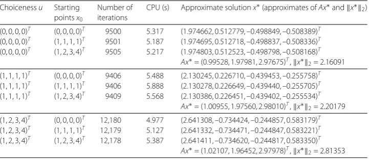
Table 1 Results for Example 5.3 using the algorithm in Corollary 3.4
Choicenessu Starting pointsx0
Number of iterations
CPU (s) Approximate solutionx∗(approximates ofAx∗andx∗2)
(0, 0, 0, 0)T (0, 0, 0, 0)T 9500 5.317 (1.974662, 0.512779, –0.498849, –0.508389)T
(0, 0, 0, 0)T (1, 1, 1, 1)T 9501 5.187 (1.974695, 0.512718, –0.498837, –0.508336)T
(0, 0, 0, 0)T (1, 2, 3, 4)T 9505 5.217 (1.974803, 0.512523, –0.498798, –0.508168)T Ax∗= (0.99528, 1.97981, 2.97675)T,x∗2= 2.16091
(1, 1, 1, 1)T (0, 0, 0, 0)T 9406 5.488 (2.130245, 0.226710, –0.439453, –0.255758)T
(1, 1, 1, 1)T (1, 1, 1, 1)T 9406 5.888 (2.130278, 0.226649, –0.439440, –0.255705)T
(1, 1, 1, 1)T (1, 2, 3, 4)T 9409 5.568 (2.130386, 0.226451, –0.439402, –0.255534)T Ax∗= (1.00955, 1.97560, 2.98010)T,x∗2= 2.20179
(1, 2, 3, 4)T (0, 0, 0, 0)T 12,180 4.977 (2.641308, –0.734424, –0.244857, 0.583179)T (1, 2, 3, 4)T (1, 1, 1, 1)T 12,179 5.127 (2.641332, –0.734471, –0.244847, 0.583221)T (1, 2, 3, 4)T (1, 2, 3, 4)T 12,178 5.387 (2.641411, –0.734620, –0.244817, 0.583350)T
Ax∗= (1.02107, 1.96452, 2.97978)T,x∗
2= 2.81353
and
h(x) =u
for allx∈R4into Corollary 3.4, we have
⎧ ⎨ ⎩
x0∈R4 chosen arbitrarily,
xn+1=αnxn+βnu+γnPC(xn–λn(A∗Axn–A∗b)), ∀n= 0, 1, 2, . . . ,
whereb= (1, 2, 3)T,λ
n= Axn–b
2
2A∗Axn–A∗b2+2A∗Axn–A∗b+Axn–b2 ifAxn= bandλn= 0 ifAxn=b for alln= 0, 1, 2, . . . . Asn→ ∞, we havexn→x∗such thatx∗is the our solution, which de-pends on the pointuandx0. The numerical results are listed in Table 1 using the different
pointsuand the different starting pointsx0.
Example5.4 (A split feasibility problem) Let
A= ⎛ ⎜ ⎝
2 –1 3
4 2 5
2 0 2
⎞ ⎟
⎠, C=(x,y,z)∈R3:x+y2+ 2z≤0
and
Q=(x,y,z)∈R3:x2+y–z≤0. Find some pointx∗∈CwithAx∗∈Q.
LetH= (R3, ·
2) andK= (R3, · 2). Takec(x,y,z) =x+y2+ 2z,q(x,y,z) =x2+y–z
andh(x,y,z) = 0 for allx,y,z∈Rinto Corollary 4.2, we have ⎧
⎨ ⎩
x0∈R3 chosen arbitrarily,
xn+1=αnxn+γnPCn(xn–λn(A∗Axn–A∗PQn(Axn))), ∀n= 0, 1, 2, . . . ,
whereλn= Axn–PQn(Axn)
2
2A∗Axn–A∗PQn(Axn)2+2A∗Axn–A∗P
Qn(Axn)+Axn–PQn(Axn)2 ifAxn∈/ Qnandλn= 0 if
Table 2 Results for Example 5.4 using Qu and Xiu method in [7]
Starting pointsx0 Number of iterations
CPU (s) Approximate solutionx∗ Approximate ofc(x∗)
Approximate ofq(Ax∗)
(1, 2, 3, 0, 0, 0)T 1890 2.7740 (–0.1203, 0.0285, 0.0582)T –0.00308775 –0.0152279
(1, 1, 1, 1, 1, 1)T 2978 4.2860 (0.8603, –0.1658, –0.5073)T –0.12681 1.08162
[image:19.595.116.481.190.246.2](1, 2, 3, 4, 5, 6)T 3317 4.8570 (3.6522, –0.1526, –2.3719)T –1.06831 15.5579
Table 3 Results for Example 5.4 using Qu and Xiu method in [6]
Starting pointsx0 Number of iterations
CPU (s) Approximate solutionx∗ Approximate ofc(x∗)
Approximate ofq(Ax∗)
(1, 2, 3)T 64 0.1570 (–0.4019, 0.0674, 0.1967)T –0.00395724 0.0322236
(1, 1, 1)T 81 0.0940 (0.3568, 0.0343, –0.2652)T –0.172424 0.426806
rand(3, 1)∗10 105 0.0940 (0.8747, 0.0795, –0.6876)T –0.49418 1.5322
Table 4 Results for Example 5.4 using Li method in Algorithm 1 [8]
Starting pointsx0 Number of iterations
CPU (s) Approximate solutionx∗ Approximate ofc(x∗)
Approximate ofq(Ax∗)
(1, 2, 3)T 4 0.1410 (–0.4024, 0.0658, 0.1958)T –0.00647036 0.0319258
(1, 1, 1)T 5 0.0940 (0.3532, 0.0392, –0.2707)T –0.186663 0.43465
rand(3, 1)∗10 8 0.0940 (0.8768, 0.0604, –0.6844)T –0.488352 1.51358
Table 5 Results for Example 5.4 using Algorithm in Corollary 4.2
Starting pointsx0 Number of iterations
CPU (s) Approximate solutionx∗ Approximate ofc(x∗)
Approximate ofq(Ax∗)
(1, 2, 3)T 1220 1.492 (–0.0009, 0.0007, 0.0002)T –0.00049951 0.00050081
(1, 1, 1)T 1062 1.342 (0.0004, 0.0007, –0.0006)T –0.00079951 0.00130016
(4, 5, 6)T 1225 1.642 (0.0006, 0.0007, –0.0007)T –0.00079951 0.00140036
rand(3, 1)∗10 1197 1.832 (0.0008, 0.0004, –0.0007)T –0.00059984 0.00110064
(6, 5, 4)T 2569 4.346 (0.0020, 0.0004, –0.0015)T –0.00099984 0.00190400
(2, 2, 2)T 1365 2.083 (0.0007, 0.0006, –0.0008)T –0.00089964 0.00140049
(3, 2, 1)T 2093 3.525 (0.0015, 0.0005, –0.0013)T –0.00109975 0.00180225
which depends on the zero point andx0. The numerical results are listed in Table 5 using
the different starting pointsx0, and we compare the results of Qu and Xiu [6, 7], and Li
[8], which are listed in Table 2, Table 3 and Table 4, respectively. We found that in the calculation approximate value ofq(Ax∗) using the our algorithm method was fit to the solution than the algorithms method of Qu and Xiu, and Li.
Example5.5 (A convex feasibility problem) LetC={a∈R3: 2≤ a2≤3}. Find some
pointx∗∈Cwhich satisfies the following system of nonlinear inequalities: ⎧
⎨ ⎩
y2+z2– 4≤0,
–x2+z– 1≤0,
wherex,y,z∈R. LetH= (R3, ·
2),K= (R3, · 2) andu∈C. TakeA=I,h(x,y,z) =uand
C=(x,y,z)∈R3:c(x,y,z) =supc1(x,y,z),c2(x,y,z)
≤0,
Q=(x,y,z)∈R3:q(x,y,z) =supq1(x,y,z),q2(x,y,z)
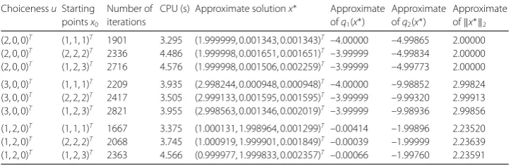
[image:19.595.115.480.281.338.2] [image:19.595.117.478.372.472.2]Table 6 Results for Example 5.5 using Algorithm in Corollary 4.2
ChoicenessuStarting pointsx0
Number of iterations
CPU (s) Approximate solutionx∗ Approximate ofq1(x∗)
Approximate ofq2(x∗)
Approximate ofx∗2
(2, 0, 0)T (1, 1, 1)T 1901 3.295 (1.999999, 0.001343, 0.001343)T –4.00000 –4.99865 2.00000 (2, 0, 0)T (2, 2, 2)T 2336 4.486 (1.999998, 0.001651, 0.001651)T –3.99999 –4.99834 2.00000 (2, 0, 0)T (1, 2, 3)T 2716 4.576 (1.999998, 0.001506, 0.002259)T –3.99999 –4.99773 2.00000
(3, 0, 0)T (1, 1, 1)T 2209 3.935 (2.998244, 0.000948, 0.000948)T –4.00000 –9.98852 2.99824 (3, 0, 0)T (2, 2, 2)T 2417 3.505 (2.999133, 0.001595, 0.001595)T –3.99999 –9.99320 2.99913 (3, 0, 0)T (1, 2, 3)T 2821 3.955 (2.998563, 0.001346, 0.002019)T –3.99999 –9.98936 2.99856
(1, 2, 0)T (1, 1, 1)T 1667 3.375 (1.000131, 1.998964, 0.001299)T –0.00414 –1.99896 2.23520 (1, 2, 0)T (2, 2, 2)T 2068 3.745 (1.000919, 1.999901, 0.001849)T –0.00039 –1.99999 2.23639 (1, 2, 0)T (1, 2, 3)T 2363 4.566 (0.999977, 1.999833, 0.002357)T –0.00066 –1.99760 2.23591
such thatc1(x,y,z) =x2+y2+z2– 9,c2(x,y,z) = –x2–y2–z2+ 4,q1(x,y,z) =y2+z2– 4 and
q2(x,y,z) = –x2+z– 1 for allx,y,z∈Rinto Corollary 4.2, we have
⎧ ⎨ ⎩
x0∈R3 chosen arbitrarily,
xn+1=αnxn+βnu+γnPCn(xn–λn(xn–PQnxn)), ∀n= 0, 1, 2, . . . ,
whereλn=
xn–PQnxn
3xn–PQnxn+2 for alln= 0, 1, 2, . . . . Asn→ ∞, we havexn→x∗such thatx∗is
the our solution, which depends on the pointuandx0. The numerical results are listed in
Table 6 using the different pointsu∈Cand the different starting pointsx0.
Example5.6 (A convex minimization problem) Find minimize of f(x,y,z) = (x– 2)2+ (y– 2)2+ (z– 3)2subject to the constraintg(x,y,z) =x2+y2+z2– 4 = 0 wherex,y,z∈R.
Define the Lagrange functionL(x,y,z,λ) as follows:
L(x,y,z,λ) =f(x,y,z) +λg(x,y,z)
= (x– 2)2+ (y– 2)2+ (z– 3)2+λx2+y2+z2– 4,
where x,y,z,λ∈R. Hence, the our solution set is equivalent to the solution set of the following system of nonlinear equations:
⎧ ⎪ ⎪ ⎪ ⎪ ⎪ ⎨ ⎪ ⎪ ⎪ ⎪ ⎪ ⎩
2(x– 2) + 2λx=Lx= 0, 2(y– 2) + 2λy=Ly= 0, 2(z– 3) + 2λz=Lz= 0,
x2+y2+z2– 4 =L
λ= 0.
LetH= (R4, ·
2) andK= (R4, · 2). TakeA=I,h(x,y,z,λ) = 0 and
C=(x,y,z,λ)∈R4:c(x,y,z,λ) = sup
1≤i≤4
–qi(x,y,z,λ)≤0
,
Q=
(x,y,z,λ)∈R4:q(x,y,z,λ) = sup
1≤i≤4
qi(x,y,z,λ)≤0
,
such that
q1(x,y,z,λ) = 2(x– 2) + 2λx, q2(x,y,z,λ) = 2(y– 2) + 2λy,
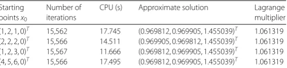
Table 7 Results for Example 5.6 using Algorithm in Corollary 4.2
Starting pointsx0
Number of iterations
CPU (s) Approximate solution Lagrange
multiplier
(1, 2, 1, 0)T 15,562 17.745 (0.969812, 0.969905, 1.455039)T 1.061319
(2, 2, 2, 0)T 15,566 14.511 (0.969905, 0.969812, 1.455039)T 1.061319
(1, 2, 3, 0)T 15,567 11.666 (0.969812, 0.969905, 1.455039)T 1.061319
(4, 5, 6, 0)T 15,566 17.495 (0.969812, 0.969905, 1.455039)T 1.061319
for allx,y,z,λ∈Rinto Corollary 4.2, we have ⎧
⎨ ⎩
x0∈R4 chosen arbitrarily,
xn+1=αnxn+γnPCn(xn–λn(xn–PQnxn)), ∀n= 0, 1, 2, . . . ,
whereλn=
xn–PQnxn
3xn–PQnxn+2 for alln= 0, 1, 2, . . . . Asn→ ∞, we havexn→x∗ such that the
our solution is √2
17(2, 2, 3)
Twith some Lagrange multiplierλ, which depends on the zero point andx0. The numerical results are listed in Table 7 using the different starting points
x0, and we switch the stopping criterionto 10–4for the verification to the our solution.
6 Conclusion
In this paper, we obtain an iterative scheme using the gradient projection method with a new step size, which is not depend on the related matrix inverses and the largest eigen-value (or the spectral radius of the self-adjoint operator) of the related matrix, based on Moudafi’s viscosity approximation method for solving thesplit common fixed point prob-lem (SCFP) for two firmly nonexpansive mappings and also solving thesplit feasibility problem(SFP) such that other strong convergence theorems for the SCFP and the SFP are obtained.
Acknowledgements
The author would like to thank the Faculty of Science, Maejo University for its financial support.
Competing interests
The author declares that he has no competing interests.
Authors’ contributions
The author read and approved the final manuscript.
Publisher’s Note
Springer Nature remains neutral with regard to jurisdictional claims in published maps and institutional affiliations.
Received: 12 December 2017 Accepted: 10 May 2018 References
1. Tian, M., Zhang, H.F.: Regularized gradient-projection methods for finding the minimum-norm solution of the constrained convex minimization problem. J. Inequal. Appl.2017, Article ID 13 (2017)
2. Tang, J.F., Chang, S.S., Liu, M.: General split feasibility problems for families of nonexpansive mappings in Hilbert spaces. Acta Math. Sci.36B(2), 602–613 (2016)
3. Censor, Y., Elfving, T.: A multiprojection algorithm using Bregman projections in a product space. Numer. Algorithms
8, 221–239 (1994)
4. Byrne, C.: Iterative oblique projection onto convex sets and the split feasibility problem. Inverse Probl.18, 441–453 (2002)
5. Yang, Q.Z.: The relaxedCQalgorithm solving the split feasibility problem. Inverse Probl.20, 1261–1266 (2004) 6. Qu, B., Xiu, N.H.: A note on theCQalgorithm for the split feasibility problem. Inverse Probl.21, 1655–1665 (2005) 7. Qu, B., Xiu, N.H.: A new halfspace-relaxation projection method for the split feasibility problem. Linear Algebra Appl.
428, 1218–1229 (2008)
![Table 2 Results for Example 5.4 using Qu and Xiu method in [7]](https://thumb-us.123doks.com/thumbv2/123dok_us/235260.1022858/19.595.117.478.372.472/table-results-example-using-qu-and-xiu-method.webp)