An Advanced Iterative Method Based on Intelligent Determination of Recurrences

An Advanced Iterative Method Based on

Intelligent Determination of Recurrences

Moe Thuthu

_{Seiji Fujino}

_{Yusuke Onoue}

Abstract— In general the product-type iterative methods utilize three-term recurrences only in its al-gorithm for accleration of convergence rate. However, computational cost of three-term recurrences, i.e., computation of inner products, needs large amount. Accordingly it is crucial for us to devise an efficient iterative method using partly two-term recurrences without degradation of convergence rate. In this pa-per, we propose an advanced GPBiCG AR2 method by means of intelligent determination of two-term or three-term recurrences.

Keywords: GPBi-CG method, GPBiCG AR method, Two-term recurrences, Three-term recurrences, ad-vanced GPBiCG AR2 method

1

Introduction

Generalized Product Bi-Conjugate Gradient (abbrevi-ated as GPBi-CG) method [8] is an attractive iterative method for the solution of a linear system of equations with nonsymmetric coefficient matrix. However, the pop-ularity of GPBi-CG method has diminished over time ex-cept for the context of limited field of analysis because of instability of convergence rate. Therefore some versions of GPBi-CG method which have stability of convergence compared with the original GPBi-CG method have been proposed.

We proposed a safety variant (abbreviated as BiCGSafe) of Generalized Product type Bi-CG method from the viewpoint of reconstruction of the residual polynomial and determination of two acceleration parametersζ_nand

ηn [2]. It embodied that a particular strategy for

reme-dying the instability of convergence, acceleration parame-ters are decided from minimization of the associate resid-ual of 2-norm [6]. However, we could not reveal the origin of instability of GPBi-CG method because of reconstruc-tion of the algorithm. Though both convergence rate and stability of BiCGSafe method were improved, instability itself of GPBi-CG method could not corresponds directly to its algorithm.

∗_{Graduate School of Information Science and Electrical}

Engi-neering, Kyushu University, Email: [email protected]

†_{Research Institute for Information Technology, Kyushu}

Univer-sity, Email: [email protected]

‡_{Graduate School of Information Science and Electrical}

Engi-neering, Kyushu University, Email: [email protected]

As a result, we proposed the original GPBiCG AR (GP-BiCG with Associate Residual) method [3] in 2007, and could verify robustness of GPBiCG AR method. Moreover, we proposed simple variant of GPBiCG AR2 method to improve convergence rate. That is, in simple variant of GPBiCG AR2 method, three-term recurrences are adopted for odd iteration steps and two-term recur-rences are adopted for even iteration steps, one after the other. This remedy makes enhancement of convergence rate of GPBiCG AR method at fairly satisfied degree. However, sometimes this remedy has a limitation of en-hancement to a certain extent.

This paper is organized as follows. In section 2 we briefly review GPBi-CG and GPBiCG AR methods. In section 3 we consider on coeffcients of GPBi-CG like methods. In particular, we propose simple and advanced variants of GPBiCG AR method by means of improvement of intelligent determination of coefficients ζ_n, η_n. In sec-tion 4 we verify effectiveness of advanced variant of GP-BiCG AR2 method with parameterκthrough numerical experiments. In section 5 we draw some concluding re-marks.

2

GPBiCG AR method

We consider iterative methods for solving a linear system of equations

Ax=b (1)

whereA∈RN×N is a given nonsymmetric matrix, andx,

bis a solution vector and right-hand side vector, respec-tively. WhenAis a large, sparse matrix which arises from realistic problems, the efficient solution of (1) is substan-tially very difficult. This difficulty has led to the devel-opment of a rich variety of generalized CG type methods having varying degrees of success (see, e.g., [7]).

cases but fail in others heightens the need for further in-sight and development of the Lanczos type iterative meth-ods. We note that the basic recurrence relations between Lanczos polynomialsR_n(λ) andP_n(λ) hold as follows:

R0(λ) = 1, P0(λ) = 1, (2)

Rn+1(λ) = Rn(λ)−αnλPn(λ), (3)

Pn+1(λ) = Rn+1(λ) +βnPn(λ), n= 1,2, . . . . (4)

Then we can introduce the three-term recurrence rela-tions for Lanczos polynomialsR_n(λ) only by eliminating

Pn(λ) from (2) and (4) as follows:

R0(λ) = 1, R1(λ) = (1−α0λ)R0(λ) (5)

Rn+1(λ) = (1 +_αβn−1

n−1αn−αnλ)Rn(λ)

−β_αn−1

n−1αnRn−1(λ), n= 1,2, . . . (6)

GPBi-CG method[8] was discovered that an often excel-lent convergence property can be gained by choosing for acceleration polynomials H_n(λ) that are built up in the three-term recurrence form as polynomial R_n(λ) in (5) and (6) by adding suitable undetermined parameters ζ_n andη_n as follows:

H0(λ) = 1, H1(λ) = (1−ζ0λ)H0(λ), (7)

Hn+1(λ) = (1 +ηn−ζnλ)Hn(λ)−ηnHn−1(λ), (8)

n= 1,2, . . . .

The polynomialsH_n(λ) satisfy H_n(0) = 1 and the rela-tion asH_n+1(0)−H_n(0) = 0 for alln. Here we introduce an auxiliary polynomialsG_n(λ) as

Gn(λ) := Hn(λ)−_ζ Hn+1(λ)

nλ . (9)

By reconstruction of (6) using the acceleration polyno-mials H_n(λ) and G_n(λ), we have the following coupled two-term recursion of the form as

H0(λ) = 1, G₀(λ) =ζ₀, (10)

Hn(λ) = Hn−1(λ)−λGn−1(λ), (11) Gn(λ) = ζnHn(λ) +ηnGn−1(λ), (12)

n= 1,2, . . . .

Using these acceleration polynomials H_n(λ) andG_n(λ), his discover led to the generalized product-type methods based on Bi-CG method for solving the linear system with nonsymmetric coefficient matrix. He refered as GPBi-CG

method [8]. However, the original Lanczos algorithm is also known to break down or nearly break down in some cases. In practice, the occurrence of a break down cause failure to converge to the solution of linear equations, and the increase of the iterations introduce numerical error into the approximate solution. Therefore, convergence of the generalized product-type methods is affected. Com-paratively little is known about the theoretical properties of the generalized product-type methods. The fact that the generalized product-type methods perform very well in some cases but fail in others motivates the need for further insight into the construction of polynomials for the product-type residualH_n+1(λ)R_n+1(λ).

In a usual approach, acceleration parameters are de-cided from local minimization of the residual vector of 2-norm ||rn₊₁(:= H_n+1(λ)R_n+1(λ))||₂, where R_n+1(λ) denotes the residual polynomial of Lanczos algorithm and

Hn+1(λ) denotes the acceleration polynomial for

conver-gence. Instead, it embodies that a particular strategy for remedying the instability of convergence. That is, the algorithm of GPBiCG AR method based on local min-imization of associate residual a r_n(:= H_n+1(λ)R_n(λ)) with two parametersζ_n andη_n is written as follows:

a rn=rn−η_nAzn₋₁−ζ_nArn. (13) Here rn is the residual vector of the algorithm. Matrix-vector multiplication ofAunandArn₊₁are directly com-puted according to definition of multiplication of matrix

A and vector. On the other hand, Ap_n and Azn are computed using its recurrence. In the algorithm of GP-BiCG AR method, modification parts which differ from the conventional GPBi-CG method are indicated with underlines. The description as computeAu_n means that multiplication of matrixAand vectoru_n asAu_n is done according to multiplication’s definition. The algorithm of the original GPBiCG AR method are written as follows:

x0 is an initial guess, r0=b−Ax0,

chooser∗₀ such that (r∗₀, r₀)= 0,

setβ₋₁= 0, computeAr₀,

forn= 0,1,· · · until||rn₊₁|| ≤ε||r₀|| do :

begin

p_n=rn+β_n−1(p_n−1−un₋₁),

Ap_n=Ar_n+β_n−1(Ap_n−1−Au_n−1),

αn= (r

∗

0,rn)

(r∗₀, Ap_n),

an=rn, bn=Azn₋₁, cn=Arn,

ζn= (bn,bn)(cn,an)−(bn,an)(cn,bn) (cn,cn)(bn,bn)−(bn,cn)(cn,bn),

ηn= (cn,cn)(bn,an)−(bn,cn)(cn,an) (c_n,c_n)(b_n,b_n)−(b_n,c_n)(c_n,b_n),

(if n= 0, thenζ_n= (cn,an)

un=ζ_nAp_n+η_n(tn₋₁−rn+β_n−1un₋₁), computeAu_n,

tn=rn−α_nAp_n,

zn =ζnrn+ηnzn₋₁−αnun,

Azn=ζnArn+ηnAzn−1−αnAun, xn+1=xn+αnp_n+zn,

rn+1=tn−Azn,

computeArn₊₁,

βn= α_ζn

n ·

(r∗₀,r_n+1) (r∗₀,rn) , end

3

Intelligent

determination

of

coeffi-cients

3.1

GPBi-CG

Coefficientsζ_n,η_n are computed for every iteration step by means of local minimization of 2-norm of residual

rn+1:=H_n+1(λ)R_n+1(λ).

an=tn, bn=yn, cn=Atn, (14)

ζn= (₍b_cn,bn)(cn,an)−(bn,an)(cn,bn)

n,cn)(bn,bn)−(bn,cn)(cn,bn), (15)

ηn= (₍c_cn,cn)(bn,an)−(bn,cn)(cn,an)

n,cn)(bn,bn)−(bn,cn)(cn,bn). (16)

However, residual vectorr_n+1 and solution vectorx_n+1 are derived from reccurences with different root, respec-tively.

tn =rn−α_nAp_n, (17)

rn+1=tn−ζnAtn−ηnyn,

(=t_n−Az_n) (18)

xn+1=xn+αnp_n+zn. (19)

Because coefficients ζ_n, η_n are designed so as to be in-cluded in the recurrence of residual vectorr_n+1. Accord-ingly solution vectorxn₊₁may differ from residual vector

rn+1 during iteration steps.

3.2

GPBiCG AR

Coefficientsζ_n,η_n are computed for every iteration step by means of local minimization of 2-norm of associate residualar_n+1(=r_n−η_nAz_n−1−ζ_nAr_n).

an=rn, bn=Azn₋₁, cn=Arn, (20)

ζn= eqn.(15), ηn = eqn.(16) (21)

On the contrary, in GPBiCG AR, both residual vector

rn+1 and solution vector xn+1 are derived from

recur-rence with the same root as below.

tn =rn−α_nAp_n, (22)

xn+1=xn+αnp_n+zn, (23)

rn+1=tn−Azn. (24)

However, coefficientsζ_n,η_nare not included in the recur-rence of residual vectorrn₊₁ itself. Therefore, we adopt an associate residual vectorarn₊₁:=H_n+1(λ)R_n(λ) for determination of ζ_n,η_n.

3.3

Variants of GPBiCG AR2

Coefficients ζ_n, η_n of simple variant of GPBiCG AR2 method are decided as below.

if step is even number, then

ζn= eqn.(15), η_n= eqn.(16) else (i.e., step is odd number)

ζn= (₍c_cnn,_,a_cnn₎), ηn = 0,

end if

Coefficientsζ_n,η_n of advanced variant of GPBiCG AR2 method are decided as below. κis given as 0 < κ≤1.0 for taking account of effect of term of η_nAzn₋₁.

ρ= |(an,cn)| ||an|| ||cn||, if ρ < κ, then

ζn= eqn.(15), ηn = eqn.(16)

else

ζn= (cn,an)

(c_n,c_n), ηn= 0, end if

Criterion as |(an,cn)|

||an|| ||cn|| =

|(rn,Arn)|

||rn|| ||Arn|| < κ based on Ref.[5], is introduced in place of odd or even number of iteration steps. Parameterκis a scalar value included in [0,1]. This variant of GPBiCG AR2 method with alter-native recurrences is refered to as an_{advanced variant}

of GPBiCG AR2 method with parameter κ. The al-gorithm of advanced variant of GPBiCG AR2 method is listed as follows:

x0 is an initial guess, r₀=b−Ax₀, chooser∗₀ such that (r∗₀, r₀)= 0,

setβ₋₁= 0, κis given as 0< κ≤1,

computeAr₀,

forn= 0,1,· · · until||r_n+1|| ≤ε||r₀||do :

begin

p_n=r_n+β_n−1(p_n−1−u_n−1),

αn = (r

∗

0,rn)

(r∗₀, Ap_n),

an =rn, bn =Azn₋₁, cn =Arn,

ρ= |(an,cn)| ||an|| ||cn||, if ρ < κ, then

ζn =(bn,bn)(cn,an)−(bn,an)(cn,bn) (c_n,c_n)(b_n,b_n)−(b_n,c_n)(c_n,b_n),

ηn =(₍c_cnn,_,c_cnn)(₎₍b_bnn,_,a_bnn₎)−₋₍(b_bnn_,,_cncn₎₍)(_cncn,_,a_bnn₎), un=ζnApn+ηn(tn−1−rn+βn−1un−1),

computeAun,

tn=rn−αnApn,

zn=ζ_nrn+ηnzn₋₁−αnun,

Azn=ζ_nArn+η_nAzn₋₁−α_nAun, else

ζn =(cn,an)

(c_n,c_n), ηn= 0,

un=ζnApn,

computeAun,

tn=rn−α_nAp_n,

zn=ζntn,

Azn=ζ_nArn−α_nAun, end if

xn+1=xn+αnpn+zn, rn+1=tn−Azn,

computeAr_n+1,

βn =α_ζn

n ·

(r∗₀,r_n+1) (r∗₀,r_n) , end

4

Numerical experiments

In this section numerical experiments will be presented. All computations were done in double precision float-ing point arithmetics, and performed on HP workstation xw4200 with CPU of Intel(R) Pentium (R) 4, clock of 3.9GHz, main memory of 3GB, OS of Suse Linux version 9.2. Compile option with “-O3” is used. The right-hand side b was imposed from the physical load conditions. The stopping criterion for successful convergence of the iterative methods is less than 10−7of the relative residual 2-norm||rn₊₁||₂/||r₀||₂. The maximum number of itera-tions is fixed as 104. The initial shadow residualr∗₀is set as the initial residualr₀(=b−Ax₀). Parameterκvaries from 0.0 to 1.0 at the interval of 0.05. In Table 1 we show chacteristics of test matrices. These test matrices are derived from Florida sparse matrix collection[1]. In Table 1, n, nnz and ave. nnz denote dimension of ma-trix, total number of nonzero entries and average number of nonzero enties per one row, respectively. The symbol “∞” means breakdown during iteration process.

Table 1: The chacteristics of test matrices.

matrix n nnz ave. analytic

nnz field

big 13,209 91,465 6.92 structural sme3Da 12,504 874,887 69.97 structural sme3Db 29,067 2,081,063 71.60 structural xenon1 48,600 1,181,120 24.30 structural comsol 9,801 48,609 4.96 structural 0 0 100 9,801 48,609 4.96 structural 0 0 200 39,601 197,209 4.98 structural 2007OK01 54,903 3,990,483 72.68 structural wang3 26,064 177,168 6.80 electrial wang4 26,068 177,196 6.80 electrial memplus 17,758 126,150 7.10 electrial 2D bjtcai 27,628 442,898 16.03 semiconduc. 3D 3D 51,448 1,056,610 20.54 semiconduc. nmos3 18,588 386,594 20.80 semiconduc. ex11 16,614 1,096,948 66.03 hydro dynamic ex19 12,005 259,879 21.65 hydro dynamic epb1 14,734 95,053 6.45 thermal epb2 25,228 175,027 6.94 thermal epb3 84,617 463,625 5.48 thermal poisson3da 13,514 352,762 26.10 poisson p poisson3db 85,623 2,374,949 27.74 poisson p fidap035 19,716 218,308 11.07 fluid dynamic af23560 23,560 484,256 20.55 fluid dynamic

Table 2: Iterations, computation times and time ratios of advanced variant of GPBiCG AR2 method withκto

time of GPBi-CG and GPBiCG AR methods.

matrix GP AR advanced AR2

itr. time itr. time itr. time opt. ratio to

[s] [s] [s] κ GP AR

comsol 261 0.22 255 0.21 215 0.17 .30 0.77 0.81 sme3Db 4612 95.65 4738 96.94 3893 79.74 .55 0.83 0.82 memplus 624 1.47 601 1.32 514 1.10 .40 0.75 0.83 sme3Da 5410 43.54 4028 31.98 3469 27.66 .95 0.64 0.86 wang3 187 0.69 181 0.62 166 0.54 .20 0.78 0.87 epb1 347 0.62 351 0.58 346 0.51 .05 0.82 0.88 0 0 100 105 0.10 100 0.09 100 0.08 .55 0.80 0.89 2D bjtcai 4058 22.31 3818 19.73 3430 17.48 .20 0.78 0.89 af23560 1942 10.15 2058 10.18 1829 9.08 .80 0.89 0.89 xenon1 488 6.59 521 6.67 468 5.98 .50 0.91 0.90 wang4 398 1.44 395 1.31 363 1.21 .85 0.84 0.92 ns3Da 739 11.93 767 12.16 70011.16 .50 0.94 0.92 poisson3db 161 6.73 162 6.53 156 6.05 .45 0.90 0.93 0 0 200 207 1.13 204 1.02 197 0.96 .95 0.85 0.94 epb2 230 0.79 239 0.77 231 0.73 .70 0.92 0.95 3D 3D ∞ ∞6344 75.88 6102 72.08 .20 – 0.95 ex19 2237 5.96 2218 5.69 2098 5.44 .15 0.91 0.96 2007OK01 1839 57.74 1866 57.39 180255.31 .55 0.96 0.96 poisson3da 87 0.35 90 0.36 89 0.35 .45 1.00 0.97 epb3 2866 37.09 2647 30.79 2678 30.07 .15 0.81 0.98 ex11 981 8.13 917 7.57 901 7.45 .95 0.92 0.98 fidap035 1053 3.37 923 2.83 932 2.82 .40 0.84 1.00 big 2528 4.17 2235 3.412235 3.47 1.0 0.83 1.02

shown in the most right column implies computation time of advanced variant of GPBiCG AR2 method with opti-mumκto the original GPBi-CG and GPBiCG AR meth-ods. The values of advanced variant of GPBiCG AR2 method represents those of the least computation time. From Table 2, we can understand that advanced variant of GPBiCG AR2 method with optimum κ outperforms well compared with other iterative methods.

0 0.2 0.4 0.6 0.8 1

0 0.1 0.2 0.3 0.4 0.5 0.6 0.7 0.8 0.9 1 17 19 21 23 25

Ratio of two-term recurrence

Time [s]

kappa

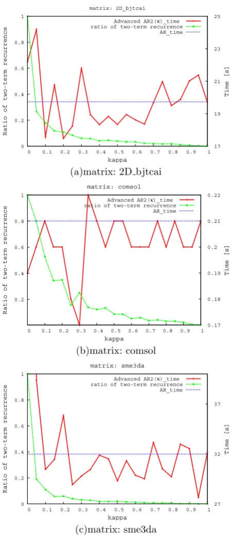
matrix: 2D_bjtcai

Advanced AR2(κ)_time ratio of two-term recurrence AR_time

(a)matrix: 2D bjtcai

0.2 0.4 0.6 0.8 1

0 0.1 0.2 0.3 0.4 0.5 0.6 0.7 0.8 0.9 1 0.17 0.18 0.19 0.2 0.21 0.22

Ratio of two-term recurrence

Time [s]

kappa matrix: comsol

Advanced AR2(κ)_time ratio of two-term recurrence AR_time

(b)matrix: comsol

0 0.2 0.4 0.6 0.8 1

0 0.1 0.2 0.3 0.4 0.5 0.6 0.7 0.8 0.9 1 27 32 37

Ratio of two-term recurrence

Time [s]

kappa matrix: sme3da

Advanced AR2(κ)_time ratio of two-term recurrence AR_time

(c)matrix: sme3da

Figure 1: Variation of ratio of two-term recurrences of GPBiCG AR2 method with various values ofκ.

0.2 0.4 0.6 0.8 1

0 0.1 0.2 0.3 0.4 0.5 0.6 0.7 0.8 0.9 1 6 6.5 7 7.5 8

Ratio of two-term recurrence

Time [s]

kappa matrix: poisson3db

Advanced AR2(κ)_time ratio of two-term recurrence AR_time

(a)matrix: poisson3db

0 0.2 0.4 0.6 0.8 1

0 0.1 0.2 0.3 0.4 0.5 0.6 0.7 0.8 0.9 1 79 89 99 109 119 129

Ratio of two-term recurrence

Time [s]

kappa matrix: sme3db

Advanced AR2(κ)_time ratio of two-term recurrence AR_time

(b)matrix: sme3db

0 0.2 0.4 0.6 0.8 1

0 0.1 0.2 0.3 0.4 0.5 0.6 0.7 0.8 0.9 1 1.1 1.2 1.3 1.4 1.5

Ratio of two-term recurrence

Time [s]

kappa matrix: memplus

Advanced AR2(κ)_time ratio of two-term recurrence AR_time

(c)matrix: mumplus

Figure 2: Variation of ratio of two-term recurrences of GPBiCG AR2 method with various values ofκ. (cont’d)

axis means ratio of two-term recurrence of advanced GP-BiCG AR2 method. Horizontal axis means values of pa-rameter κ. From Figs.1-2, it can be seen that advanced GPBiCG AR2 method with κ works well exception for very small values of parameterκ.

Figs.3 (a)-(d) exhibit history of relative residual 2-norm of GPBiCG (in pink dotted line), GPBiCG AR (in blue dashed line with mark “ ”) and advanced variant of GP-BiCG AR2 (in red solid line) methods. From Fig.3, it can be made clear that advanced variant of GPBiCG AR2 method has the most excellence of robust convergence rate.

5

Concluding remarks

The advanced variant of GPBiCG AR2 method outper-forms well compared with the conventional GPBi-CG, GPBiCG AR and simple variant of GPBiCG AR2 meth-ods. A future work is to choose an optimum κfor each matrix. Moreover, it is crucial to examine the relation-ship between κ used in BiCGStab method [5] and that used in GPBiCG AR method.

References

[1] Florida sparse matrix collection: http://www.cise. ufl.edu/research/sparse/matrices/

[2] S. Fujino, M. Fujiwara and M. Yoshida: BiCGSafe method based on minimization of associate residual, Transaction of JSCES 2005. (in Japanese)

[3] Moe Thuthu, S. Fujino: Stability of GPBiCG AR method based on minimization of associate resid-ual, The Abstract of Asian Symposium on Computer Mathematics, December 2007, Singapore.

[4] Moe Thuthu, S. Fujino: Stability of GPBiCG AR method based on minimization of associate residual, Transaction of ASCM, 5081(2008), 108-120.

[5] G. Sleijpen, H. van der Vorst: Maintaining conver-gence properties of BiCGstab methods in finite pre-cision arithmetic, Numerical Algorithms, ₁₀(1995), pp.203-223.

[6] H.A. van der Vorst: Bi-CGSTAB: A fast and smoothly converging variant of Bi-CG for the solu-tion of nonsymmetric linear systems, SIAM J. Sci. Stat. Comput.,₁₃(1992), 631-644.

[7] H.A. van der Vorst: Iterative Krylov precondition-ings for large linear systems, Cambridge University Press, Cambridge, 2003.

[8] S.-L. Zhang: GPBi-CG: Generalized product-type preconditionings based on Bi-CG for solving non-symmetric linear systems, SIAM J. Sci. Comput.,

18(1997), 537-551.

-7 -6 -5 -4 -3 -2 -1 0 1

0 100 200 300 400 500 600

Relative Residual

Iterations matrix: memplus

Advanced AR2(κ) AR GP

(a)matrix: memplus at kappa = 0.4

-7 -6 -5 -4 -3 -2 -1 0 1 2 3

0 1000 2000 3000 4000 5000

Relative Residual

Iterations matrix: sme3da

Advanced AR2(κ) AR GP

(b)matrix: sme3da at kappa = 0.95

-7 -6 -5 -4 -3 -2 -1 0 1

0 1000 2000 3000 4000 5000

Relative Residual

Iterations matrix: sme3db

Advanced AR2(κ) AR GP

(c)matrix: sme3db at kappa = 0.55

-7 -6 -5 -4 -3 -2 -1 0 1

0 50 100 150 200 250

Relative Residual

Iterations matrix: comsol

Advanced AR2(κ) AR GP

(d)matrix: comsol at kappa = 0.3