Efficient Complex Continuous-Time IIR Filter Design via Generalized Vector Fitting

Efficient Complex Continuous-Time IIR Filter

Design via Generalized Vector Fitting

Chi-Un Lei, Chung-Man Cheung, Hing-Kit Kwan and Ngai Wong

Abstract—We present a novel model identifica-tion technique for designing complex infinite-impulse-response (IIR) continuous-time filters through gen-eralizing the Vector Fitting (VF) algorithm, which is extensively used for continuous-time frequency-domain rational approximation to symmetric func-tions, to asymmetrical cases. VF involves a two-step pole refinement process based on a linear least-squares solve and an eigenvalue problem. The pro-posed algorithm has lower complexity than conven-tional schemes by designing complex continuous-time filtersdirectly. Numerical examples demonstrate that VF achieves highly efficient and accurate approxi-mation to arbitrary asymmetric complex filter re-sponses. The promising results can be realized for high-dynamic frequency range networks.

Keywords: Complex filter, Vector Fitting, Rational

Function Approximation

1

Introduction

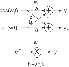
Complex signal processing has growing importance in high-speed communication systems [1, 2]. This can be seen, for example, by the majority of the LAN wire-less transceivers papers in IEEE International Solid-State Circuits Conference (2001-2003) and recent papers [3, 4]. The topology of a complex signal processing block com-prises two parallel paths, namely, an in-phase path and a quadrature path. The two cross-coupling paths have equal magnitude gain but have π/2 phase difference, as in Fig. 1. Modern wireless systems make use of this prop-erty in the design of quadrature receivers for image rejec-tion in intermediate frequency (IF), and suppression of out-of-band signals and interferences [1]. This paper re-visits and explores the design of complex continuous-time filters.

Existing complex infinite-impulse-response (IIR) continuous-time filter design algorithms include the first-order frequency transformation of a real lowpass filter [5], which usually results in a high-order filter due to unnecessary coefficient symmetry. In [2] and [6], algorithms are proposed to combine real filter design and conformal mapping to eliminate such transformation.

∗_{Department of Electrical and Electronic Engineering, The} Uni-versity of Hong Kong, Pokfulam Road, Hong Kong. Email: {culei, edmondcheung, kwanhk, nwong}@eee.hku.hk

+

+

X

a

a

b

b

-y

y

cos(w

t)

sin(w

t)

K=a+jb

y

e

(a)

(b) jw_it

Figure 1: (a) The real signal-flow graph (SFG) of a com-plex multiply and (b) the equivalent comcom-plex SFG.

However, both methods can only approximate a single passband response (but not arbitrary, say, multiple pass-band response) and do not consider phase matching and efficient design for advanced and adaptive applications.

On the other hand, a continuous-time frequency-domain system identification technique, known as Vector Fitting (VF) [7], is a robust macromodeling tool for fitting sam-pled frequency data with a rational function. Its ex-tensive applications include power system modelling [8] and high-speed VLSI interconnect simulations [9]. Its counterpart, called discrete-time vector fitting (VFz), has been adapted to real digital filter design in [10] with remarkable performance. However, traditional VF has been restricted to symmetric functions. In this paper, VF is adapted to asymmetric functions for complex IIR continuous-time filter design.

2

Vector Fitting

In complex filter design, the ultimate goal is to ap-proximate a prescribed asymmetric frequency-domain re-sponse by a complex transfer function:

f(s) =H0 M Q i=1

(s−βi)

N Q i=1

(s−αi)

, (1)

where H0 ∈ ℜ and αi, βi ∈ C. f(s) is the desired

fre-quency response, H0, αi, βi, M and N represent gain,

poles, zeros, the number of zeros and the number of poles, respectively.

To fit the continuous-time rational function, Vector Fit-ting (VF) [7] attempts to reformulate (1) into partial frac-tion basis:

f(s) = (

N X

n=1

cn

s−an

) +d+se, (2)

to a set of calculated/sampled data points at frequencies

{sk}, for k = 1,2,· · · , Ns. In real response

approxima-tion of VF, the polesan and residuescn are real or

com-plex conjugate pairs. In comcom-plex filtering, this restriction is relaxed and VF readily handles complex poles and ze-ros arising in this stage. The constant termdand eare generally complex.

2.1

Problem Formulation

The fitting process begins with specifying an initial set of pole{α(0)n }. By introducing of the scaling functionσ(s),

a linear problem is set up for theith iteration, namely

N X

n=1

cn

s−α(i)n !

+d+se

| {z }

(σf)(s)

≈

_N

X

n=1

γn

s−α(i)n !

+ 1

!

| {z }

σ(s)

f(s),

(3)

for i = 0,1,· · · , NT, where NT denotes the number of

iterations when convergence is attained or when the up-per limit is reached. The unknowns,cn,d,eandγn, are

solved through an overdetermined linear equation formed by evaluating (3) at the Ns sampled frequency points.

One important feature in (3) is that (σf)(s) andσ(s)f(s) are enforced to share the same set of poles, which in turn implies that the original poles of f(s) are cancelled by the zeros ofσ(s). And the relationship can be described as follows:

N_Q+1

n=1

s−βn(i)

N Q n=1

s−α(i)n

| {z }

(σf)(s)

≈

N+1_Q

n=1

s−βe(i)n

N Q n=1

s−α(i)n

| {z }

σ(s)

f(s), (4)

⇒f(s)≈ (σf) (s)

σ(s) =

N+1_Q

n=1

s−β(i)n

N+1_Q

n=1

s−βe(i)n

. (5)

Subsequently, solving the zeros of σ(s), in the least-squares sense, results in an approximation to the poles of f(s), i.e., {α(i+1)n }, without restriction of real

coeffi-cients. The new poles are then fed back to (3) as the next set of known poles for further refinement iteratively. In practical implementation, the fitting equation in (3) is linear in its unknowns cn, d and γn. Therefore, the

non-linear problem can be solved using over-determined equations and eigenvalue solving.

2.2

Pole Calculation

At a particular frequency point, withe = 0, (3) becomes

N X

n=1

cn

sk−α(i)n !

+d−

N X

n=1

γnf(sk)

sk−α(i)n !

≈f(sk), (6)

it can be reformulated into:

Akx=bk, (7)

where x = c1 · · · cN 1 γ1 · · · γN T

, Ak =

h ₁

sk−α(1i)

· · · 1

sk−α(Ni)

d −f(sk)

sk−α(1i)

· · · −f(sk)

sk−α(Ni)

i

andbk=f(sk).

In the above expression, Ak and xare row and column

vectors, respectively, whilebk is a scalar.

Equating (7) at all frequency samples, mathematically sk =jΩk, fork= 1,2,· · ·, NS, whereNS >2N+ 1, and

by stackingAk’s andbk’s into a (tall) column matrix and

a vector, an overdetermined equation for theith iteration is obtained:

Ax=b. (8)

The scaling functionσ(s) in (3) can be reconstructed from the last N entries obtained from the least-squares solu-tion (i.e.,γ1,γ2,· · ·,γN inx), such that its zeros,{α(i+1)n },

forn= 1,2,· · · , N, are taken as the new set of starting poles in the next VF iteration. Moreover, it can be shown that{α(i+1)n }are conveniently computed as the

Ψ =       α( i) 1 α( i) 2 . ._. α( i) N       −      1 1 . . . 1     

γ1 γ2 · · · γN

.

(9)

Since the poles are not restricted to complex-conjugate pairs, Ψ is generally a complex matrix. Upon conver-gence, the update inα(i)n diminishes and σ(s)≈1.

To ensure system stability, it is necessary that Reα(i+1)n

< 0. If this is not the case, any unstable pole is flipped about the imaginary axis to the open left half plane Reα(i+1)n

:= −Reα(i+1)n

. Such stability enforcement has the physical meaning of multiplying all-pass filters onto the filter transfer function such that the magnitude response is preserved.

2.3

Building the Rational Function

Once a converged set of poles {α(NT)

n } is obtained, the

final stage is to reconstruct the rational function complex IIR filter. Referring to (3), we should now haveσ(s)≈1 so that

N X

n=1

cn

s−α(NT)

n !

+d≈f(sk), (10)

for k= 1,2,· · · , Ns. The residuescn ofF(s) are

deter-mined exactly in the same manner, except (7) is replaced as follows:

Akx=bk, (11)

where x= c1 · · · cN 1 T

, bk =f(sk) and Ak =

h ₁

sk−α(1i)

· · · 1

sk−α(Ni)

d i_{.The summation of partial}

fractions

_N

P n=1

cn

s−α(nNT)

+dgenerates a rational function

representing the complex IIR filter in the form of (2). By seeking a near-optimal fit tof(sk) [5], VF matches both

magnitude and phase off(sk) simultaneously.

In summary, comparing to VF, other complex IIR de-sign algorithms such as the pole-placement algorithm in [2] give similiar accuracy but has much higher com-putational requirement and does not emphasize the im-portance of phase linearity. For high-order filter design, it was claimed that 10-15 seconds are required on a 3-GHz computer [2], in great contrast to the 1-2 seconds by our design methodology implemented on a 1.8-GHz computer. In comparison to [2] and other complex filter design algorithms, VF is superior in terms of the phase linearity in passband and much higher efficiency, as will be seen in our numerical examples.

3

Remarks

3.1

Numerical consideration

Recent research has shown that VF is in fact a reformu-lation of the Sanathanan-Koerner (SK) iteration [11], an iterative continuous-time frequency-domain system iden-tification technique [12], which minimizes the following objective function: Ns P k=0 N(

i)_(s k)

D(i

−1)(sk)−

D(i)_(s

k)

D(i

−1)(sk)f(sk)

2 = Ns P k=0 N P n=1 cn

sk+α(

i₋1)

n − 1 + N P n=1 γn

sk+α(

i₋1) n

f(sk) 2 , (12)

whereN(i)_,D(i)_{are the numerator and denominator}

de-termined during the ith iteration. In theory, the ap-proximation converges for a noise-free model using (12), but some numerical errors occur during iterative calcu-lation [15]. Therefore, numerical considerations for im-proving the approximation accuracy are highlighted:

1. The approximation accuracy in noisy environment (e.g., finite precision) is affected by the equation normalization in the original VF. Furthermore, the normalization also gives a biased approximation in the low frequency region [13]. Recently, a relaxation is proposed to improve the normalization situation. Firstly, the unity basis in (3) is replaced by a variable and a relaxation constraint,

Re

(_Ns

X k=0 1 + N X n=1 γn

sk+α(i)n !)

=Ns+ 1, (13)

is introduced in (8) with a row weighting of

kf(s)k/(Ns+ 1). As shown in [14], this relaxation

outperforms other relaxation approaches.

2. The conditioning and the approximant accuracy are affected by the choices of function basis and the lo-cation of initial-poles (i.e. α(0)n in (3)). In [7], it is

recommended that the initial poles should be dis-tributed over the frequency range of interest. As a rule of thumb in VF, the complex design algorithm starts with complex conjugate poles based on the following relationship:

an=−α+jβ, an+1=−α−jβ, (14)

Table 1: Approximation errors in the numerical exam-ples.

Ex 1. (VF) Ex 1. ( [2]) Ex. 2

L2passband 0.0124 0.0234 0.0083

L∞passband 0.0071 0.0126 0.0022

L2stopband 0.9975 1.0000 0.0068

L∞stopband 5.1452 5.1953 0.0029

technique from linear algerba [17] is used in system equation calculation to improve the numerical con-ditioning, and gives a similar accuracy as using the orthonormal basis.

3.2

Further extension

BesidesL2norm minimization, some filter design requires

equiripple passband to minimize the maximum error of a filter. In IIR digital filter design, an equiripple filter can be designed by a weighted least-squares method with a suitable least-squares frequency response weighting func-tion [18]. The idea can be extended into complex filter design, and the frequency weighting can be included using row weighting in a particular frequency-data row of (7).

4

Numerical Examples

The performance of VF in direct complex IIR filter design is illustrated by two examples run in the MATLAB 7.1 environment on a 512-RAM 1.8-GHz PC.

4.1

Example 1

In this example, we design a single-passband positive passband filter (PPF), which is widely used in communi-cation systems (e.g. single-side-band communicommuni-cation [1]). The specification is extracted from [2]. The response is sampled at 40 linearly spaced points in the passband, and 80 uniform sampling points in each stopband. The passband spans [−10,10].

Vector fitting constrains the numerator and denominator of the transfer function to have the same order. An 8-pole (8-zero) complex IIR filter was designed via VF to fit the prescribed response. It takes 0.9063 seconds for the system poles to attain convergence in 5 pole refining iter-ations. The frequency response and the passband group delay (the change of phase) are shown in Fig. 2. It can be observed that VF achieves an excellent fitting to both desired magnitude and phase response. TheL2norm and

L∞norm errors in magnitude of solution are summarized

in Table 1. The numerical example is compared with [2], and is shown by Fig. 2. It can be concluded that the phase response matches the desired constant group de-lay (i.e. linear passband) with a significantly improved computation complexity and better approximation in the

−100 −5 0 5 10

0.2 0.4 0.6 0.8 1

Frequency (Hz)

Magnitude

(a)

VF [2]

0.8 1 1.2 1.4 1.6 1.8 2 2.2 0.98

0.985 0.99 0.995 1 1.005 1.01

Frequency (Hz)

Magnitude

(b)

VF [2]

1.1 1.2 1.3 1.4 1.5 1.6 1.7 1.8 6

8 10 12 14 16 18

Frequency (Hz)

Group Delay

(c)

VF [2]

Figure 2: Frequency response of Example 1. (a) Magni-tude in the entire band, (b) magniMagni-tude in the passband and (c) group delay in the passband.

−0.8 −0.7 −0.6 −0.5 −0.4 −0.3 −0.2 −0.1 0 −10

−8 −6 −4 −2 0 2 4 6 8 10

Real

Imag

Initial Poles Final Poles

passband, with a slightly better stopband design. Fig. 3 shows the initial and final system poles.

4.2

Example 2

The second example demonstrates the versatility of the VF algorithm through the design of a wide-frequency-range double-passband complex filter, which can be used in low-IF architecture [1]. The specifications are as fol-lows:

Hd(ejω) =           

−60dBejωD_{, (−10f}

s≤ω≤ −7fs)

0dBejωD_{, (−6f}

s≤ω≤ −4fs)

−60dBejωD_{, (−3f}

s≤ω≤fs)

0dBejωD_{, (2f}

s≤ω≤6fs)

−60dBejωD_{, (7f}

s≤ω≤ −10fs)

(15)

whereDis the group delay. To illustrate the capability of VF to design wide frequency range filters, we take fs in

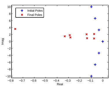
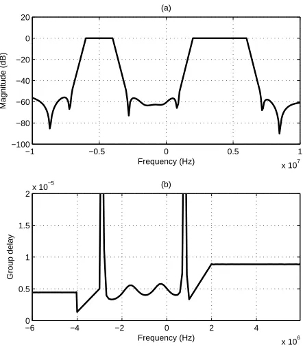
the GHz. Uniform sampling points of 80 and 40 are used in each passband and stopband respectively, i.e., 280 pling points in total. The transition bands are not sam-pled as a way of relaxation. We set the group delay to be 10 microseconds in both the passband and stopband. To approximate the desired response, a 20th-order IIR filter is designed via the VF algorithm with the numeri-cal enhancements in Section 3.1. The set of system poles converges in only 4 iterations, taking 0.8063 seconds for computation. From Fig. 4 and Table 1, the complex IIR filter via VF matches the desired magnitude response and phase linearity well over a wide frequency range. The lo-cation of initial assigned poles and converged poles in the s-plane is plotted in Fig. 5. It is noticeable that the poles are roughly located separately into two elliptical regions, each of them corresponding to a passband. Fig. 6 shows theL2error and the condition number in (3) during each

iteration. Both quantities show a significant descending trend for each iteration and converge within a few itera-tions, and in fact converge much faster than the original VF. It also shows the numerical improvement using row scaling technique.

Acknowledgment

This work was supported in part by the Hong Kong Re-search Grants Council and the University ReRe-search Com-mittee of The University of Hong Kong.

5

Conclusions

This paper has generalized VF to the design of arbitrary response complex IIR continuous-time filters. With-out symmetry constraints, the proposed method demon-strates its efficacy in producing low-order approximation functions to the desired magnitude responses over a wide frequency range with matching of phase linearity. Arbi-trary response approximation, passband phase matching,

−1 −0.5 0 0.5 1

x 107 −100

−80 −60 −40 −20 0 20

Frequency (Hz)

Magnitude (dB)

(a)

−6 −4 −2 0 2 4

x 106 0

0.5 1 1.5

2x 10 −5

Frequency (Hz)

Group delay

(b)

Figure 4: Frequency response of Example 2. (a) Magni-tude, (b) Group delay in passband.

−6 −5 −4 −3 −2 −1 0 x 105 −1

−0.8 −0.6 −0.4 −0.2 0 0.2 0.4 0.6 0.8 1

x 107

Real

Imag

Initial Poles Final Poles

Figure 5: Initial pole placement and final pole locations in Example 2.

0 5 10

0 10 20 30 40 50 60 70

No. of Iterations

Conditional Number

(a)

0 5 10

−40 −30 −20 −10 0 10

No. of Iterations

L2−norm error

(b)

and the algorithm effectiveness are definite advantages over existing methods. Different enhancement techniques are applied in the numerical computation. Numerical ex-amples have confirmed the superiority of VF over con-ventional complex IIR filter design algorithms.

References

[1] K. W. Martin, “Complex signal processing is not complex,” IEEE Trans. Circuits Syst. I, vol. 51, no. 9, pp. 1823–1836, 2004.

[2] K. W. Martin, “Approximation of complex IIR bandpass filters without arithmetic symmetry,”

IEEE Trans Circuits Syst. I, vol. 52, no. 4, pp. 794– 803, Apr. 2005.

[3] J. Mahattanakul and P. Khumsat, “Structure of complex elliptic Gm-C filters suitable for fully differ-ential implementation,”IEE Proceedings - Circuits, Devices and Systems, vol. 1, no. 4, pp. 275–282, Aug. 2007.

[4] B. Pandita and K. W. Martin, “Designing Complex delta-sigma Modulators with Signal-Transfer Func-tions having Good Stop-Band Attenuation,” inProc. IEEE Symp. Circuits and Systems, May 2007, pp. 3626–3629.

[5] A. Krukowski and I. Kate, “DSP system design: complexity reduced IIR filter implementation for practical application,” 2003.

[6] M. A. Teplechuk and J. I. Sewell, “Approximation of arbitrary complex filter responses and their real-isation in log domain,” IEE Proceedings - Circuits, Devices and Systems, vol. 153, no. 6, pp. 583–590, Dec. 2006.

[7] B. Gustavsen and A. Semlyen, “Rational approxi-mation of frequency domain responses by vector fit-ting,” IEEE Trans. Power Delivery, vol. 14, no. 3, pp. 1052–1061, July 1999.

[8] B. Gustavsen, “Wide band modeling of power trans-formers,” IEEE Trans. Power Delivery, vol. 19, no. 1, pp. 414–422, Jan. 2004.

[9] E. P. Li, E. X. Liu, L. W. Li, and M. S. Leong, “A coupled efficient and systematic full-wave time-domain macromodeling and circuit simulation method for signal integrity analysis of high-speed interconnects,” IEEE Trans. Antennas Propagat., vol. 27, no. 1, pp. 213–223, Feb. 2004.

[10] N. Wong and C. Lei, “FIR filter approximation by IIR filters based on discrete-time vector fitting,” in

Proc. IEEE Symp. Circuits and Systems, May 2007, pp. 2343–2346.

[11] W. Hendrickx and T. Dhaene, “A discussion of ”Rational approximation of frequency domain re-sponses by vector fitting”,” IEEE Trans. Power Syst., vol. 21, no. 1, pp. 441–443, Feb. 2006. [12] C. Sanathanan and J. Koerner, “Transfer function

synthesis as a ratio of two complex polynomials,”

IEEE Trans. Automat. Contr., vol. 8, no. 1, pp. 56– 58, Jan. 1963.

[13] B. Gustavsen, “Improving the pole relocating prop-erties of vector fitting,” IEEE Trans. Power Deliv-ery, vol. 21, no. 3, pp. 1587–1592, July 2006. [14] D. Deschrijver, M. Schoeman, T. Dhaene, and

P. Meyer, “Experimental analysis on the relaxation of macromodeling methods,” inProc. IEEE Africon conference, Sept. 2007.

[15] D. Deschrijver, B. Haegeman, and T. Dhaene, “Or-thonormal vector fitting: A robust macromodeling tool for rational approximation of frequency domain responses,”IEEE Trans. Adv. Packag., vol. 30, no. 2, pp. 216–225, May 2007.

[16] Y. S. Mekonnen and J. E. Schutt-Aine, “Broadband macromodeling of sampled frequency data using z-domain vector-fitting method,” inProc. IEEE work-shop on sig. prop. on interconnects, May 2007. [17] G. H. Golub and C. F. V. Loan, Matrix

Computa-tions, 3rd ed. London: Johns-Hopkins, 1996. [18] T. Kobayashi and S. Imai, “Design of IIR digital