Using a Multiple Linear Regression Model to
Calculate Stock Market Volatility
Timothy A. Smith#1, with Alex Caligiuri & J Rhet Montana Embry Riddle Aeronautical University
600 S. Clyde Morris Blvd. Daytona Beach, FL 32114 U.S.A
Abstract In mathematical finance, regression models can be used to determine the value of an asset based on its underlying traits and/or returns relative to the overall market performance. In prior work [6-7] a regression model was created to predict the value of the S&P 500 based on macroeconomic indicators. In the current study the model is updated with the addition of recent data, and then applied to define a new measure to model market volatility. The results are compared to the S&P 500’s implied volatility in a simulation utilizing the Black-Sholes model attempting to predict the value of the S&P 500 one year in the future. While no definition could be expected to perfectly predict the market volatility, the new definitions of volatility did outperform the currently utilized implied volatility.
Keywords — Partial differential equations, regression analysis, stochastic, financial mathematics. AMS classification: 35K10.
I. INTRODUCTION
It is well known that mathematical financial prediction models, such as the famous Black Scholes Stochastic Partial Differential Equation [1],
have demonstrated a limitation to perform during times of rapidly changing of volatility [2-3]. For example, in non-rapidly changing times of market valuation, hence low volatility time periods, the famous Black Scholes Formula - using the notation of T for the call option maturity date , k for the strike price, r for the risk free interest rate, and N(z) for the standard normal distribution - will accurately predict the fair price of an option. The Black Sholes Formula, with initial stock price xo, will give the fair price of the option as
“expected value” of the market based off of its fundamentals, and the true value of the S&P 500 at the given time as the “observed value” of the market. The residual of these values are then scaled so that the new volatility models can be inputted into the Black-Scholes Model for volatility, σ. This new value of volatility, along with VIX separately, are used to calculate the value of at the money S&P 500 call options expiring in exactly one year through a simulation. Hence, a fair value of the S&P 500 is computed for one year forward, and the results are compared for both values of volatility with the results showing the new measure of volatility performing better.
II. REGRESSION MODEL
A widely accepted principle in the economic and financial world is the fact that various economic indicators are correlated to the market and can be used to forecast the stock market. An original study [5] identified that the variables of consumer price index (CPI), producer price index (PPI), gross domestic product (GDP), money supply (MS), and treasury spread (T) could be used in a multiple linear regression model to explain market (S&P 500) returns and movements. This assumes that there is a linear relationship between the S&P 500 and the aforementioned independent variables. This initial model was created using monthly data from 1974 - 2005 and yielded acceptable preliminary results; however, tests for multicollinearity were not conducted, which left much room for improvement in the model and further study.
The format of this model follows that of a normal multiple linear regression model with the form
where y is the dependent variable (S&P 500), and the usual notation is utilized for the input variables and corresponding coefficients. Following the prior research [6-8] on the subject of creating a multiple linear regression model to predict the price of the S&P 500, some important results are necessary to be taken into account for the current study. The major finding of these previous studies is the finding of substantial
multicollinearity between CPI and GDP. Due to this multicollinearity that exists it becomes necessary to remove one of the two variables to improve the model and eliminate any unintended chaotic behaviour. After following routine regression coefficient analysis the variables of CPI, PPI and T were removed. At that point further data study was conducted to see if any other predictor variables could be introduced to improve the model overall; the variables were selected through a common sense approach as to what factors one would expect to predict the market, such as: the price of gasoline, or the price of boring money, or the unemployment rate etc. The final model contained variables GDP, MS, and Unemployment Rate (UI). This model was both the most statistically significant and computationally efficient model generated.
The indicators used in this new model date back to roughly 1960, however since the goal of this study was to create a new volatility model to compare with VIX, the date that the data set of our new model begins at was restricted to January 1991. This was chosen as the calculation methodology changed for the VIX in 1990, hence we started at the beginning of the closest calendar year. Taking monthly data points starting January 1st 1991 and ending December 31st 2017 yields 324 total data points for the model, with the opportunity to update the data set at any given time. The data collected was then normalized using a Z-Score transformation. The governing equation of the model over this time frame is
where Z1 corresponds to GDP, Z2 corresponds to MS, and Z3 corresponds to UI. In this model i = 1,2, … , n corresponds to the month starting with i = 1 being January 1991.
Coefficients t Stat
Intercept 1188.91 163.37
GDP 198.84 6.04
MS 298.79 9.03
ANOVA
df MS F
Regression 3 2.9E+07 1664.048
Residual 320 17159.6
Total 323
Regression Statistics
Multiple R 0.96941254
R Square 0.93976068
Figure 1. The data analysis of the updated three variable model.
As one can see above, the model has a very solid F-Statistic along with a great R2 value of 0.94. This shows that the updated multiple linear regression model is not only statistically significant, it is also a more computationally efficient model than the original model from [5].
Figure 2. A graphical representation of the models
500 to be the expected value of the market at any given time, and the actual value of the S&P 500 is considered the corresponding observed value of the market. Using these considerations, we are defining two new definitions for volatility to be compared with VIX. The calculation for the two new volatility models are very similar, as the only difference between the two formulas is whether the denominator for the volatility equation has the observed or expected value for the S&P 500 in the denominator. The full calculation for the new volatility model is the square root of the squared residual of the observed and expected value of the S&P 500 divided by either the observed S&P 500 price or the expected S&P 500 price. The residual was squared and subsequently taken the square root of to ensure that every value will be positive. These values were then multiplied by 100 in order to scale them so they could be compared with VIX. To differentiate the two models, we will consider the volatility model with the observed S&P 500 price in the denominator to be VOL1, and the model with expected S&P 500 price in the denominator to be ALTVOL.
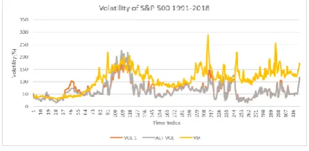
A volatility value for each model was created at each of the 324 monthly data points from the multiple regression model, and then plotted against VIX for analysis, as show below in Figure 3.
Figure 3. A graph of the volatilities raw values.
After completing a graphical analysis on Figure 3, the main takeaway is that the values for VIX over time are generally much greater than the values of the new volatility models VOL1 and ALTVOL, especially during times of calmness when there should not be a significant amount of volatility in the market. Conversely, VOL1 and ALTVOL only spike in value when the deviations between expected and observed S&P 500 prices increase, which is expected. However, the deviation between observed and expected prices primarily increases at times where the market is increasing at a rate faster than the economy is growing, creating a bubble, which will subsequently be followed by a crash in the near future. Intuitively, that scenario is when levels of volatility should be at its highest, and models VOL1 and ALTVOL are at their maximum during these periods, specifically the 2000-2002 bubble and subsequent crash.
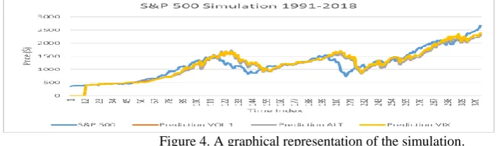
Figure 4. A graphical representation of the simulation.
The results of the simulation were mixed and there are many important key takeaways to understand. As with any financial forecast, the probability of achieving a perfect prediction are close to zero. With that in mind, the new volatility models performance in the simulation can be considered acceptable. The areas of largest difference for the simulation and actual S&P 500 occur at the times of the 2002 and 2008 financial crises. Furthermore, the VIX generally had the greatest predicted value, which supports the findings from the analysis of the volatility models. When computing the squared residuals for the simulations versus the actual S&P 500, VOL1 had the lowest value, followed by ALTVOL and VIX respectively. While the sum of the residuals squared for each simulation were high in value, the significant difference in the sum of the squared residuals between VOL1 and VIX brings proof to the claim that VIX may not be the best instrument to measure volatility in the market; hence, it is reasonable to conclude that the new volatility models fared better in a simulation due to lower overall error.
IV.CONCLUSIONS &SUGGESTION FURTHER STUDY
In this work a prior regression model was updated to contain more recent data. This model was proven to be statistically significant and justified further research using the model. One can see through comparison of the model S&P 500 and actual S&P 500 that in 2000 the market increased at a rate that the underlying economic fundamentals could not support, with a subsequent crash following in 2002, likewise for the 2008 “great recession.” In this work three volatility models were then tested in a simulation setting to see which could best predict the price of the S&P 500 one year in advance. While none of the three models performed great, the main takeaway from the simulation is that the new models we created, VOL1 and ALTVOL, both outperformed the VIX in terms of error during the observed time period.
Many complex mathematical models have been created in an attempt to accurately calculate volatility, and in this study two new definitions for volatility were created. In a prior study [6], it was suggested to create these new volatility models and input their values into the Black-Scholes formula. The results from performing this simulation showed that over time, the new volatility models outperformed VIX, especially during times of market turbulence, when volatility should be at its greatest levels. These findings provide proof to the claim that VIX is not the best way to define market volatility. It is suggested in a future study to attempt to use these new volatility models to conduct more predictions for the S&P 500, perhaps by using a shorter time to expiry on the options price calculations, say one month instead of one year. Another suggestion for further study is to research how one could apply this method to individual sectors or stocks, perhaps constructing a model that utilizes various website’s APIs in real time to collect specific data. While volatility is and will continue to be one of the most mysterious aspects in the financial world, further research into these new volatility models may yield some promising results for the future of volatility and market forecasting.
REFERENCES
[1] Black, F. and Scholes, M. “The Pricing of Options and Corporate Liabilities,” Journal of Political Economy 81 (3), 1973.
[2] Colander, David and Föllmer, Hans and Haas, Armin and Goldberg, Michael D. and Juselius, Katarina and Kirman, Alan and Lux, Thomas and Sloth, Birgitte, “The Financial Crisis and the Systemic Failure of Academic Economics.” Univ. of Copenhagen Dept. of Economics Discussion Paper No. 09-03, (2009)
[3] Moyaert, T. & Petitjean, M . “The performance of popular stochastic volatility option pricing models during the subprime crisis.” Applied Financial Economics. 21(14), 2011.
[4] Summa, John; Option Volatiliy: Historical Volatility, Investopedia (2007) [5] Park, Sam. “Reducing the Noise in Forecasting the SP 500,” Wentworth, 2005.