A Multi-Stage Adaptive Pool Testing Model with Test Errors Vis-a-Vis the Non-Adaptive Model without Test Errors

(1)

A MULTI-STAGE ADAPTIVE POOL TESTING MODEL WITH TEST ERRORS VIS-A-VIS THE NON-ADAPTIVE MODEL WITHOUT TEST ERRORS

Okoth Annette W. Department of Mathematics

Masinde Muliro University of Science and Technology P.O Box 190-50100, Kakamega, Kenya

Email:[email protected]/[email protected]

Abstract

Pool testing for presence or absence of a trait is less expensive, less time consum-ing and therefore more cost effective. This study presents a multi-stage adaptive pool testing estimator ˆpn of prevalence of a trait in the presence of test errors. An

increase in the number of stages improves the efficiency of the estimator, hence con-struction of a multi-stage model. The study made use of the Maximum Likelihood Estimate (MLE) method and Martingale method to obtain the adaptive estimator and Cramer-Rao lower bound method to determine the variance of the constructed estimator. Matlab and R, statistical softwares were used for Monte-carlo simula-tion and verificasimula-tion of the model, then analysis and discussion of properties of the constructed estimator, notably efficiency in comparison with the non-adaptive estimator in the absence of test errors in the literature of pool testing done along-side provision of the confidence interval of the estimator. Results have shown that the efficiency of the multi-stage adaptive estimator in the presence of test errors is higher than that of the non-adaptive estimator in the absence of test errors. This efficiency also increases with increase in sensitivity and specificity of the test kits. This makes the multi-stage adaptive estimator in the presence of test errors better than the non-adaptive estimator in the absence of test errors, especially so that errors in experiments in our day to day encounters are inevitable.

Keywords: Pool testing, Adaptive estimator, Test errors, Confidence in-terval

A Multi-Stage Adaptive Pool Testing Model with

Test Errors Vis-a-Vis the Non-Adaptive Model

without Test Errors

(2)

MULTI-STAGE ADAPTIVE POOL TESTING MODEL WITH TEST ERRORS 1

1 Introduction

Prevalence of defective units in a large population from accurate diagnostic tests is a fundamental risk assessment and management factor [6]. Estimation of defective units one-by-one is inefficient and uneconomical, considering that in a given population only a few individuals may be defective. It is against this background that pool testing comes in handy because it is more effective, less time consuming and less expensive [3]. Pool testing occurs when units from a population are pooled and tested as a group for the presence or absence of a particular trait. It also reduces the Mean Squared Error (MSE) of the estimates, hence it is more efficient, as was established by Sobel and Ellashoff, [9]. There are two forms of pool testing namely

(i) Non-adaptive pool testing scheme

(ii) Adaptive pool testing scheme

1.1 Non-adaptive testing scheme

In this testing scheme, a large population is divided in to n groups which are then subjected to testing [3]. When tested, a group can either test positive or negative and the outcome of the test aids in constructing the non-adaptive model.

1.2 Adaptive testing scheme

In this scheme a population is divided in to n groups, which are partitioned depending on the number of stages to be considered. Predetermined parameters are used to partition the groups and the number of partitioning parameters depends on the number of stages [6]. Partitioned groups are then tested at various stages for the presence or absence of a trait and the results used to construct the adaptive model.

1.3 Introduction of the model

In this study we obtained a multi-stage adaptive estimator ˆpn of prevalence of a trait in the presence of test errors, using the maximum likelihood estimate (MLE) method and investigated its effeciency in comparison with the non-adaptive estimator in the absence of test errors. The adaptive testing scheme involves testing groups in stages and updating group sizes from one stage to the next, with the group size at a stage depending on the outcome of the test(s) at the preceding stage(s). That is testing n1 groups each of size

k1 at stage one; n2 groups each of size k2 at stage two; n3 groups each of size k3 at

stage three and so on; where k3 depends on both k1 and k2 while k2 depends on k1.

For a general adaptive scheme, at stage i ni groups each of size ki, where ki depends on ki−1, ki−2, ki−3, ...k1 are constructed. The constructed groups are then subjected

(3)

groups, ni is determined before the experiment is carried out while ki0s are sequentially determined as the experiment progresses [7].

2 Literature Review

Pool testing has been recognized as a sampling scheme that can provide substantial benefits [7]. Early application of pool testing include tests for prevalence of plant virus transmissions by insects [10] and [9] and this was one of the pioneering applications of this concept. In [3] statistical and mathematical concepts of pool testing are introduced and used to estimate the proportion of individuals infected with some disease among the US conscripts. He also derived optimum group sizes assuming that the population was large enough for the application of the binomial model and consequently realized significant savings by reducing the number of tests required. In [9] estimation in the pool testing procedure is discussed.

In the subsequent years this concept has had relevant applications in various clinical studies including psychopathology, public health and plant quarantine [1] and [2]. Alter-natively, positively pooled samples can be partitioned into relatively smaller subsets there by reducing on cost and effort, which provides obvious motive for pooling samples [6]. In [5] an estimation model based on pool testing with retesting pools that test negative is developed. Pool testing need not only be applied to population where retesting is needed [8], like in identification of disease infected individuals in a human population, but also on other populations with no intentions of retesting the individuals contributing to positive pooled samples. For instance if a bunch of food items is being tested for contamination, there may be no interest in identifying the particular items which are affected. The aim may instead be on estimating the proportion of defective items in a population or deciding that the number of positive pooled samples justifies removing a food product from the market. In another related study, bacteriological testing of egg laying hens of salmonella in Great Britain was carried out using organ cultures pooled five at a time. Individual samples contributing to positive pooled samples are not tested again . A population com-prised of birds in a hen house. If the infection was confirmed they were destroyed and compensation paid for the number of birds estimated to be uninfected [8].

In this procedure maximum likelihood estimation is applied to estimate the pro-portion and Cramer-Rao lower bound method is used to determine the variance of the estimator. In this paper, we present a multi-stage adaptive pool testing model with im-perfect tests and compare its efficiency with that of the non-adaptive model with im-perfect tests

3 Model Description Formulation and Analysis

(4)

in the absence of test errors. For a multi-stage adaptive scheme, we set n1 = λ1n,

n2 = λ2n, n3 = λ3n, ...., nn = (1 −λ1n −λ2n− ....− λn−1n) ; where λ1, λ2,... ,

λn−1 are parameters used to partition the pools; k2 depends on the outcome at stage

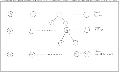
1 , k3 depends on the outcomes at stages 1 and 2 and kn depends on the outcomes at stages 1,2,3, ..., n−1 . Each constructed group at each stage is then subjected to testing, yielding either a positive or negative result. This is shown in Figure 3.1 below:

Figure 3.1: Multi-stage adaptive pool testing.

To achieve the construction of the multi-stage adaptive model in the presence of test errors, we consider two stage, three stage and four stage adaptive models in the presence of test errors and there after generalize to obtain the multi-stage model.

3.1 Two stage adaptive model

In this scheme, the population is divided into two sets of groups n1 and n2 which are

tested in two stages, with n1 groups tested at stage one and n2 groups tested at stage

two. We set n1 =λn and n2 = (1−λn) , where n is the number of groups constructed

initially. k1 which is the group size at stage one is determined by

k1 =argminl[V ar(ˆp)]|p=p0, (1)

Suppose X1 groups test positive on the test at stage-one, then

(5)

where λ is the parameter used to partition the pools while π(p) is the probability that a group is defective and is given by

π(p) := η[1−(1−p)k] + (1−φ)(1−p)k (3)

Using this model we obtain the prevalence estimator at stage one as

ˆ

p1 = 1−

"

η− X1

λn

η+φ−1 #_k1

1

, (4)

The variance of Equation (4) is similar to the variance of the non-adaptive estimator in the presence of test errors, ˆp except for K1 in place of p. This variance is given by

V ar(ˆp) = π(p)(1−π(p))

nk2₍₁₋_p₎2k−2₍_η₊_φ₋₁₎2

= (1−p)

2−2k_π₍_p₎₍₁₋_π₍_p₎₎

nk2₍_η₊_φ₋₁₎2 (5)

= (1−p)

2_π₍_p₎₍₁₋_π₍_p₎₎₍₁₋_p₎−2k

nk2₍_η₊_φ₋₁₎2

For the estimator at stage two, ˆp2, we have λn groups each of size k1 tested at stage

one and 1−λn groups each of size k2 tested at stage two. k2 is determined by

k2 =argminl[V ar(ˆp1)]|p1=p, (6)

Suppose that out of the (1−λ)n groups each of size k2 tested at stage two, X2 groups

test positive on the test, then for fixed X1 we have

X2|X1 ∼Binomial((1−λ)n, π2|1(p)) (7)

Using this model, the estimator at stage two can be obtained as the solution to

k1X1qk1[(1−φ)−η]

η−(η+ (1−φ))qk1 +

k2(X1)X2qk2(X1)[(1−φ)−η]

η−(η+ (1−φ))qk2(X1)

= k1q

k1₍_λn−_X

1)(η+ (1−φ))

1−[η−(η+ (1−φ))qk1] +

k2(X1)qk2(X1)[(1−λ)n−X2][η+ (1−φ)]

1−[η−(η+ (1−φ))qk2(X1)] .

(8)

and using cramer-Rao lower bound, its variance is obtained as

V ar(ˆp2) =

π1(p)π2(p)(1−π1(p))(1−π2(p))

A , (9)

(6)

3.2 Three stage adaptive model

Next we consider the estimator at stage three, ˆp3, where we have λ1n groups each of size

k1 tested at stage one, λ2n groups each of size k2 tested at stage two and 1−λ1n−λ2n

groups each of size k3 tested at stage three. k3 is determined by

k3 =argminl[V ar(ˆp2)]|p2=p1, (10)

If out of the (1−λ1−λ2)n groups each of size k3 tested at stage three, X3 groups test

positive on the test, then for fixed X1 and X2 we have

X3|X1, X2 ∼Binomial((1−λ1−λ2)n, π3|1,2(p)) (11)

We use this model to obtain the estimator at stage three as the solution to

k1X1qk1[(1−φ)−η]

η−(η+ (1−φ))qk1 +

k2(X1)X2qk2(X1)[(1−φ)−η]

η−(η+ (1−φ))qk2(X1) +

k3(X1, X2)X3qk3(X1,X2)[(1−φ)−η]

η−(η+ (1−φ))qk3(X1,X2)

= k1q k1₍_λ

1n−X1)(η+ (1−φ))

1−[η−(η+ (1−φ))qk1] +

k2(X1)qk2(X1)[λ2n−X2][η+ (1−φ)]

1−[η−(η+ (1−φ))qk2(X1)]

+k3(X1, X2)q

k3(X1,X2)_[(1−_λ

1−λ2)n−X3][η+ (1−φ)]

1−[η−(η+ (1−φ))qk3(X1,X2)] = 0, (12)

and its variance as

V ar(ˆp3) =

π1(p)π2(p)π3(p)(1−π1(p))(p)(1−π2(p))(p)(1−π3(p))

nB (13)

where B is defined in appendices.

3.3 Four stage and multi-stage adaptive models

Extending the notion in the above sub-sections further we have estimators at stages four and n given by solutions to

k1X1qk1[(1−φ)−η]

η−(η+ (1−φ))qk1 +

k2(X1)X2qk2(X1)[(1−φ)−η]

η−(η+ (1−φ))qk2(X1)

+k3(X1, X2)X3q

k3(X1,X2)_[(1₋_φ₎₋_η_]

η−(η+ (1−φ))qk3(X1,X2) +

k4(X1, X2, X3)X4qk4(X1,X2,X3)[(1−φ)−η]

η−(η+ (1−φ))qk4(X1,X2,X3)

= k1q k1₍_λ

1n−X1)(η+ (1−φ))

1−[η−(η+ (1−φ))qk1] +

k2(X1)qk2(X1)[λ2n−X2][η+ (1−φ)]

1−[η−(η+ (1−φ))qk2(X1)]

+k3(X1, X2)q

k3(X1,X2)_[_λ

3n−X3][η+ (1−φ)]

1−[η−(η+ (1−φ))qk3(X1,X2)_]

+k4(X1, X2, X3)q

k4(X1,X2,X3)_[(1₋_λ

1−λ2−λ3)n−X4][η+ (1−φ)]

(7)

and

k1X1qk1[(1−φ)−η]

η−(η+ (1−φ))qk1 +

k2(X1)X2qk2(X1)[(1−φ)−η]

η−(η+ (1−φ))qk2(X1) ....

+kn(X1, ..., X(n−1))Xnq

kn(X1,...,X(n−1))_[(1−_φ₎−_η_]

η−(η+ (1−φ))qkn(X1,...,X(n−1)) (15)

= k1q k1₍_λ

1n−X1)(η+ (1−φ))

1−[η−(η+ (1−φ))qk1_] +

k2(X1)qk2(X1)[λ2n−X2][η+ (1−φ)]

1−[η−(η+ (1−φ))qk2(X1)_] ...

+kn(X1, ..., X(n−1))q

kn(X1,...,X(n−1))_[(1−_λ

1−λ2)n−X4][η+ (1−φ)]

1−[η−(η+ (1−φ))qkn(X1,...,X(n−1))_] = 0,

respectively. Using Cramer-Rao lower bound method their variances are obtained as

V ar(ˆp4) =

π1(p)π2(p)π3(p)π4(p)(1−π1(p))(p)(1−π2(p))(p)(1−π3(p))(1−π4(p))

C (16)

and

V ar(ˆpn) =

π1(p)π2(p)...πn(p)(1−π1(p))(p)(1−π2(p))(p)...(1−πn(p))

D (17)

where C and D are given in the appendices respectively.

3.4 Confidence Interval(CI) of

p

ˆ

n

Next we provide the confidence interval for our multi-stage estimator, ˆpn. This confidence interval is given by

ˆ

pn +

−Zα2

p

var(ˆpn), (18)

where Zα

2 ∼N ormal(0,1) . and ˆpn and var(ˆpn) are provided by the solution to 15 and

Equation 17 respectively. It follows from Equation 18 that

p∈[ˆpn−Zα

2

p

var(ˆpn),pˆn+Zα

2

p

var(ˆpn)]

and by the law of Central Limit Theorem (CLT) we have

√

n(ˆpn−p) l

→N ormal(0,pvar(ˆpn))

or

√

n_p(ˆpn−p) var(ˆpn))

l

→N ormal(0,1).

(8)

4 Discussion of Results, Conclusion and

Recommen-dations

In this section we discuss the results as provided by Tables 4.1 , 4.2 and 4.3 and Figures 4.1 , 4.2 and 4.3 . The highlights of the results will enable us make a detailed conclusion to this study.

4.1 Discussion

Here we highlight our findings in this study. We estimated prevalence, p of a trait using the Multi-stage adaptive pool testing scheme. We accomplished this by employing the Maximum Likelihood Estimate (MLE) procedure. For us to recommend the suitability of the Multi-stage adaptive estimator, it would be in order to first compare with the non-adaptive estimator in the absence of test errors. Our measure of comparison herein is the computation of Asymptotic Relative Efficiency (ARE) values for different values of

η and φ at various stages. For simplicity of comparison and understanding, ARE values were computed for stages two to four. Upon careful analysis of the estimators at these stages, we had a good basis to make a generalization about the multi-stage estimator in the presence of test errors.

4.2 Comparing the Adaptive estimator in the presence of test

errors with the non-adaptive estimator in the absence of

test errors

We now compare our constructed estimators at stages two, three and four, that is ˆp2,

ˆ

p3 and ˆp4 with the non-adaptive estimator in the absence of test errors. According to

[?], for the non-adaptive estimator in the absence of test errors, say, ˆpe its variance is defined as

var(ˆpe) =

1−(1−p)k

nk2₍₁₋_p₎k−2 (19)

ARE values for stages two, three and four are obtained by dividing Equation (19) by Equations (9), (13) and (16) respectively. That is,

V ar(ˆpe)

V ar(ˆp2)

, V ar(ˆpe) V ar(ˆp3)

and V ar(ˆpe) V ar(ˆp4)

,

where V ar(ˆpe) , V ar(ˆp2) , V ar(ˆp3) and V ar(ˆp4) are given by Equations (19), (9), (13)

and (16) respectively. On simplifying we obtain

AREpˆ2 =

S k2₍₁₋_p₎k−2_π

1(p)π2(p)(1−π1(p))(1−π2(p))

(9)

AREpˆ3 =

T k2₍₁₋_p₎k−2_π

1(p)π2(p)π3(p)(1−π1(p))(1−π2(p))(1−π3(p))

,

AREpˆ4 =

U k2₍₁₋_p₎k−2_π

1(p)π2(p)π3(p)(1−π1(p))(1−π2(p))(1−π3(p))

,

where S, T and U are described in the appendices. Using these Equations and R-Gui software Tables 4.1 , 4.2 and 4.3 was generated.

p η=φ= 0.99 η=φ= 0.98 η=φ= 0.97 η=φ= 0.96 η=φ= 0.90

0.1 0.6201 0.5937 0.5679 0.5429 0.9733

0.2 0.9348 0.8920 0.8507 0.8107 1.0439

0.3 1.5885 1.4827 1.3853 1.2953 1.3985

0.4 3.0934 2.7607 2.4843 2.2492 2.0817

0.5 6.9677 5.7850 4.9357 4.2828 3.3723

0.6 18.6193 13.8911 10.9879 8.9982 5.9110

0.7 59.3263 36.9918 26.4215 20.2549 11.3545

0.8 202.1403 105.234 69.6775 51.2275 26.4611

0.9 922.4898 449.351 290.6582 211.1664 106.6068

Table 4.1: ARE values of pˆ2 relative to pˆ for specified p, η and φ

p η=φ= 0.99 η=φ= 0.98 η=φ= 0.97 η=φ= 0.96 η=φ= 0.90

0.1 0.6979 0.6686 0.6400 0.6121 0.4590

0.2 0.9565 0.9058 0.8578 0.8120 0,5784

0.3 1.4487 1.3245 1.2169 1.1220 0.7158

0.4 2.4726 2.1414 1.8917 1.6911 0.9626

0.5 4.4726 4.0575 3.4339 2.9648 1.4774

0.6 12.6180 9.3723 7.4005 6.0547 2.5406

0.7 39.6622 24.7168 17.6506 13.5297 4.8532

0.8 134.8077 70.1796 46.466 34.1625 11.2807

0.9 615.0049 299.5731 193.7758 140.7802 45.4864

(10)

p η =φ = 0.99 η =φ = 0.98 η=φ = 0.97 η=φ= 0.96 η=φ= 0.90

0.1 0.7753 0.7424 0.7102 0.6789 0.5076

0.2 0.9490 0.8888 0.8332 0.7816 0.5347

0.3 1.2518 1.11482 1.0049 0.9131 0.5555

0.4 1.8535 1.5650 1.3624 1.2051 0.6672

0.5 3.3923 2.7251 2.2866 1.9634 0.9654

0.6 8.1539 6.0084 4.7282 3.8611 1.6141

0.7 24.9753 15.5415 11.0927 8.5007 3.0478

0.8 84.3418 43.9045 29.0689 21.3714 7.0569

0.9 384.399 187.2438 121.116 87.9926 28.4306

Tables 4.1 , 4.2 and 4.3 provide generated ARE values for specified values of p, η

and φ at stages two, three and four. It can be noticed from the tables that the adaptive estimators at stages two, three and four, that is ˆp2, ˆp3 and ˆp4 register ARE values slightly

less than 1 at p <0.3 , except for η=φ=.90 where the efficiency is slightly less than 1 for p = 0.1 at stage two, for p < 0.5 at stage three and for p < 0.6 at stage four. This means that when prevalence is low the adaptive estimators in the presence of test errors are slightly less efficient than the non-adaptive estimator in the absence of test errors. However, the scenario changes for p > 0.2 across all stages for η = φ > .90 and for

p >0.4 for η=φ=.90 at stages three and four, as efficiency of the adaptive estimators significantly improves. Therefore, as prevalence increases, the adaptive estimators in the presence of test errors outperform the non-adaptive estimator in the absence of test errors especially when the sensitivity and specificity of test kits are high. It is also clear from the tables that ARE values increase with increase in the number of stages; the adaptive estimator at stage two having the lowest ARE values while the estimator at stage four has the highest ARE values. This is an important pointer to the fact that the adaptive testing scheme gets better as the number of stages increases.

(11)

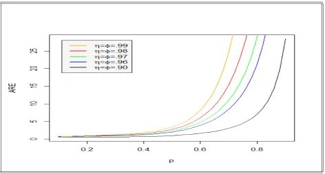
Figure 4.1: ARE of ˆp2 vs probability, p

(12)

Figures 4.1 , 4.2 and 4.3 represent ARE values plotted against prevalence p values at stages two, three and four respectively. Clearly, as noted in Tables 4.1 , 4.2 and 4.3 , the ARE values are slightly less than 1 at low values of p but increase significantly as prevalence increases. From Figures 4.1 , 4.2 and 4.3 , it is clear that the adaptive estimators outperform the non-adaptive estimator in the absence of test errors as the sensitivity and specificity of the test kit increases.

4.3 Conclusion and Recommendations

From the above discussions, it is clear that the multi-stage adaptive estimator in the presence of test errors outperforms the non-adaptive estimator in the absence of test errors. A closer look at the results reveals that the multi-stage adaptive estimator is particularly better in cases where test kits have high sensitivity and specificity. Given that experiments are never 100% perfect, the multi-stage adaptive testing scheme is therefore more ideal in estimating prevalence of a trait.

(13)

References

[1] Bhattacharyya, G.K., Karandinos, M.G., and DeFoliart, G. R. (1979). Point estimates and confidence intervals for infection rates using pooled organisms in epidemiologic studies. American journal of epidemiology109,124-131.

[2] Chiang, C. L. and Reeves, W. C. (1962). Statistical estimation of virus infection rates in mosquito vector populations. American journal on hygiene 75, 377-391

[3] Dorfman R. (1943). The detection of defective members of large populations. Annals of mathematical statistics14, 436-440.

[4] Mood, D. A., Graybill, G. A., Boes, D. C. (1974). Introduction to the theory of statistics. 27, 72.

[5] Nyongesa, L. K. (2011).Dual estimation of prevalence and disease incidence in pool testing strategy. Communication in statistics theory and methods,40, 1-12

[6] Okoth, A. W. (2012). Two Stage Adaptive Pool Testing for estimating prevalence of a trait in the presence of test errors. Lambert Academic publishers, 18 and 27

[7] Oliver-Hughes J.M. and Swallow W.H. (1994),A two-stage adaptive group testing procedure for estimating small proportions. American statistical association89, 982-993.

[8] Richards, M. S. (1991). Interpretation of the results of bacteriological testing of egg lay-ing flocks for salmonella enteritidis. Proceedings of the 6th international symposium on veterinary epidemiology and economics, 124-126, Ottawa, Canada.

[9] Sobel M., Ellashoff R.M. (1975).Group testing with a new goal; estimation. Biometrika62, 181-193.

[10] Swallow W.H. (1987).Relative MSE and cost considerations in choosing group size for group testing to estimate infection rates and probability of disease infection. Phytopathology77, 1376-1381.

(14)

Appendices

A = (η+φ−1)2n

[π2(p)(1−π2(p))λk12(1−p)2k1

−2₊_π

1(p)(1−π1(p))(1−λ)k22(X1)(1−p)2k2(X1)−2]

(21)

B = (η+φ−1)2

∗ hπ2(p)(1−π2(p))π3(p)(1−π3(p))λ1nk1(1−p)k1−2

+ π1(p)(1−π1(p))π3(p)(1−π3(p))λ2nk2(X1)(1−p)k2(X1)−2

+ π1(p)(1−π1(p))π2(p)(1−π2(p))λ2nk3(X2)(1−p)k3(X2)−2

C = (η+φ−1)2n h

π2(p)(1−π2(p))π3(p)(1−π3(p))π4(p)(1−π4(p))λ1nk1(1−p)k1−2

+ π1(p)(1−π1(p))π3(p)(1−π3(p))π4(p)(1−π4(p))λ2nk2(X1)(1−p)k2(X1)−2

+ π1(p)(1−π1(p))π2(p)(1−π2(p))π4(p)(1−π4(p))λ3nk3(X2)(1−p)k3(X2)−2

+ π1(p)(1−π1(p))π2(p)(1−π2(p))π3(p)(1−π3(p))(1−λ1−λ2−λ3)nk4(X3)(1−p)k4(X3)−2

(23)

D = (η+φ−1)2n

∗

π2(p)(1−π2(p))...πn(p)(1−πn(p))λ1nk1(1−p)k1−2

+ π1(p)(1−π1(p))...πn(p)(1−πn(p))λ2nk2(X1)(1−p)k2(X1)−2+....

+ π1(p)(1−π1(p))π2(p)(1−π2(p))...π(n−1)(p)(1−π(n−1)(p))

(1−λ1−λ2−...−λ(n−1))nkn(X(n−1))(1−p)kn(X3)−2

S = [1−(1−p)k](η+φ−1)

π2(p)(1−π2(p))λk21(1−p)2k1−2+π1(p)(1−π1(p))(1−λ)k22(X1)(1−p)2k2(X1)−2

(15)

T = [1−(1−p)k](η+φ−1)

π2(p)(1−π2(p))π3(p)(1−π3(p))λk12(1−p)2k1

−2

+ π1(p)(1−π1(p))π3(p)(1−π3(p))λ2k22(X1)(1−p)2k2(X1)−2

+ π1(p)π2(p)(1−π1(p))(1−π2(p))(1−λ1−λ2)k32(X2)(1−p)2k3(X2)−2

U = [1−(1−p)k](η+φ−1)

π2(p)π3(p)π4(p)(1−π2(p))(1−π3(p))(1−π4(p))λk12(1−p)2k1−2

+ π1(p)π3(p)π4(p)(1−π1(p))(1−π3(p))(1−π4(p))λ2k22(X1)(1−p)2k2(X1)−2

+ π1(p)π2(p)π4(p)(1−π1(p))(1−π2(p))(1−π4(p))λ3k32(X2)(1−p)2k3(X2)−2

+ π1(p)π2(p)π3(p)(1−π1(p))(1−π2(p))(1−π3(p))(1−λ1−λ2−λ3)k42(X3)(1−p)2k4(X3)−2