www.geosci-model-dev.net/5/457/2012/ doi:10.5194/gmd-5-457-2012
© Author(s) 2012. CC Attribution 3.0 License.
Geoscientific
Model Development
Detection, tracking and event localization of jet stream features in
4-D atmospheric data
S. Limbach1,2, E. Sch¨omer1, and H. Wernli2
1Institute for Computer Science, Johannes-Gutenberg University, Mainz, Germany 2Institute for Atmosphere and Climate Science, ETH, Zurich, Switzerland
Correspondence to: S. Limbach ([email protected])
Received: 1 November 2011 – Published in Geosci. Model Dev. Discuss.: 17 November 2011 Revised: 18 March 2012 – Accepted: 19 March 2012 – Published: 16 April 2012
Abstract. We introduce a novel algorithm for the efficient detection and tracking of features in spatiotemporal atmo-spheric data, as well as for the precise localization of the occurring genesis, lysis, merging and splitting events. The algorithm works on data given on a four-dimensional struc-tured grid. Feature selection and clustering are based on ad-justable local and global criteria, feature tracking is predom-inantly based on spatial overlaps of the feature’s full vol-umes. The resulting 3-D features and the identified corre-spondences between features of consecutive time steps are represented as the nodes and edges of a directed acyclic graph, the event graph. Merging and splitting events appear in the event graph as nodes with multiple incoming or out-going edges, respectively. The precise localization of the splitting events is based on a search for all grid points in-side the initial 3-D feature that have a similar distance to two successive 3-D features of the next time step. The merging event is localized analogously, operating backward in time. As a first application of our method we present a climatol-ogy of upper-tropospheric jet streams and their events, based on four-dimensional wind speed data from European Centre for Medium-Range Weather Forecasts (ECMWF) analyses. We compare our results with a climatology from a previous study, investigate the statistical distribution of the merging and splitting events, and illustrate the meteorological signif-icance of the jet splitting events with a case study. A brief outlook is given on additional potential applications of the 4-D data segmentation technique.
1 Introduction
In this introductory section we will first explain the need for and usefulness of developing efficient automated algorithms for identifying and tracking specific features of the highly variable atmospheric flow. In a second subsection, a brief review is provided of previously developed feature detection and tracking algorithms, which will serve as a basis for mo-tivating the novel approach developed in this study.
1.1 Identification and tracking of atmospheric flow features
Albeit highly variable, the atmospheric flow can be described by characteristic and frequently recurring flow features, like for instance tropopause-level jet streams, and surface cy-clones and anticycy-clones. These flow features are particu-larly important since they are typically associated with cer-tain weather conditions (e.g. sunny and dry weather with sub-tropical anticyclones; stormy weather and intense precipita-tion with extratropical cyclones) and with specific dynamical processes (e.g. cyclogenesis on the poleward side of intense upper-level jet exit regions).
Therefore, several algorithms have been developed during the last decades to objectively and efficiently identify atmo-spheric flow features from large datasets. These algorithms make it possible, for instance, to produce synoptic climatolo-gies of specific features and, if applied to homogeneous cli-mate datasets, to quantify potential trends in the frequency of these features.
climatological density maps of these features. They are typ-ically identified as local extrema of a particular field (e.g. minimum sea level pressure). The later techniques also con-sidered the temporal coherency of the features, which led to the computation of feature tracks, and feature genesis and lysis points. For a concise review on cyclone identi-fication and tracking methods, the reader is referred to Ul-brich et al. (2009). The algorithm introduced by Wernli and Schwierz (2006) considers cyclones explicitly as finite-size two-dimensional features (instead of point objects). Sim-ilar approaches have been used to identify, for instance, tropospheric jet streams (Koch et al., 2006) and upper-tropospheric cut-off cyclones (Wernli and Sprenger, 2007) as two-dimensional features. The objective identification of these features was based upon either the topology of the two-dimensional field (e.g. considering the outermost closed con-tour surrounding a local extremum) or a simple threshold (e.g. considering the region where a field exceeds a certain value). So far, all these two-dimensional feature identifica-tion algorithms have been applied to individual time steps of climatological atmospheric data (e.g. every 6 h if using re-cent reanalysis datasets) and additional tracking algorithms have been used to meaningfully connect the identified fea-tures in time. As a consequence, these feature identification and tracking algorithms treat the spatial and temporal dimen-sions of atmospheric data very differently.
In this current study we will introduce a novel approach to the identification and tracking of atmospheric flow fea-tures as full 3-D objects developing over time. In addition, our method estimates the location of the detected merging and splitting events in grid point space. The output of our segmentation method allows performing specific analyses of the interaction and development of the observed atmospheric features. For instance, a precise event localization is useful for the computation of climatologies of events and for a sta-tistical analysis of the lifetime and stability of an atmospheric feature. In addition, the location of feature events (e.g. the merging of two jet streams or the splitting of an extratropical cyclone) can objectively pinpoint important atmospheric pro-cesses. In Sect. 4.1, we will present a case study to illustrate this point.
1.2 Conceptional view on feature identification and tracking
Feature extraction and tracking are common tasks in different scientific areas, for example in image processing and com-puter vision (Zucker, 1976; Pal and Pal, 1993; Jain et al., 1995), as well as in flow visualization (see Post et al. (2003) for an overview). An important goal of feature extraction and tracking is the creation of reduced datasets and derived attributes characterizing the parts of interest of the original, often much larger input dataset. Such a reduced representa-tion allows for a statistical evaluarepresenta-tion of the features and for an efficient visualization.
Several methods for the extraction of flow features exist. The choice of a method depends considerably on the char-acteristics of the input datasets as well as on the features of interest. In Post et al. (2003), feature extraction approaches are classified into three groups: based on image processing, on topological analysis, and on physical characteristics. In our current application, we are not aiming for a topological analysis but focus on the physical characteristics of the un-derlying dataset, and on the adaption of image processing methods for our purpose.
Van Walsum (1995) proposed a feature extraction method called “selective visualization”. This method uses a boolean selection criterion for deciding whether a single grid point belongs to a feature or not, and a connectivity criterion in or-der to cluster neighboring selected points. Other approaches, for example by Reinders (2001), use this selective visual-ization method for feature extraction. Silver and Zabusky (1993) propose to apply region growing techniques for de-tecting features. Region growing is a well-known image seg-mentation technique, see, e.g. Zucker (1976). The basic idea is to start the segmentation at an initial grid point, commonly representing an extremal value of the dataset, and then to iter-atively add new neighboring grid points, as long as they can still be associated with the phenomenon to be detected. The usage of a spatial data structure, for example an octree (Silver and Zabusky, 1993; Wilhelms and Van Gelder, 1992), can be effective for speeding up the data processing. Siegesmund (2006) applied a region growing method for the segmen-tation of ozone holes from time-series of two-dimensional ozone data. Muelder and Ma (2009) let an approximation of the boundary grid points of a feature successively shrink and grow, until they obtain a new boundary representation of the feature at the next time step. Their initial approxima-tion is based upon an extrapolaapproxima-tion of the results of previ-ous time steps. For the detection of new features that may have formed, they perform a search over all unassigned grid points.
Post et al. (2003) proposed three different basic ap-proaches towards feature tracking. The first approach is to extend a three-dimensional feature detection method to the full spatiotemporal domain, as it is done for example by Wei-gle and Banks (1998), Bauer and Peikert (2002), and Ji et al. (2003). The second approach is to test features for region correspondence on a cell-to-cell basis, as proposed by Silver and Zabusky (1993), and Silver and Wang (1997, 1999). The third type of feature tracking covers methods which compare attributes of the features of consecutive time steps (for ex-ample total mass, center of mass, or moments). Samtaney et al. (1994) performed feature tracking by testing whether the differences of the observed attributes of the features stay within preassigned tolerances. Reinders (2001) used corre-spondence functions, which estimate the similarity of the at-tributes of different features for feature tracking.
atmospheric reanalysis data), we aimed for a method that ap-plies feature extraction, clustering, attribute calculation and tracking in one sequential pass over the dataset. Our method for feature extraction uses ideas from many of the approaches mentioned above. Single grid points are selected based on a local selection criterion. Clustering is performed based on a local homogeneity criterion. We decide to keep or discard single segments afterwards based on a global selection crite-rion. This compensates, to a certain extent, for the selection of a seed-point as in traditional region growing techniques. During the iteration over the data, we represent intermediate features using a union-find data structure (see, e.g. Knuth, 1997 and Cormen et al., 2009) to guarantee efficient opera-tions on the features (for example merging multiple features as soon as a connection is detected). Since we aim for the precise localization of the features and their events, we keep track of all grid points of every feature at all steps of the al-gorithm.
We realize feature tracking by testing for spatial overlap on a cell-to-cell basis. This was an obvious decision since it corresponds to a plain extension of our algorithm from three to four dimensions. We initially designed our algorithm for the detection and tracking of atmospheric features such as jet streams, which are relatively large and slow-moving with respect to the temporal resolution of our datasets. However, even in case of such features we have to deal with continua-tions of small, fast-moving features that can not be identified by spatial overlaps. To cover these cases as well, we perform additional tests for continuation based on comparisons of the center of mass and volume attributes of the features.
Our algorithm represents the temporal relations between features detected during the feature tracking in form of an event graph. An event graph is a directed acyclic graph as proposed by Samtaney et al. (1994). They identified four different events: creation, dissipation, bifurcation, and amal-gamation. In order to stay in line with the terminology used in atmospheric sciences, we call these events genesis, lysis, splitting, and merging. Our algorithm puts no additional con-straints on the detection of events and does not detect unre-solved events, in contrast to, e.g. the method by Reinders (2001).
We implemented the algorithm as part of a novel software tool for the analysis and segmentation of atmospheric data (Limbach et al., 2009). As one of our first applications, we computed a climatology of upper-tropospheric jet streams and their events, as documented in this study. The data basis of the jet stream segmentation were operational meteorolog-ical analyses from the European Center for Medium-Range Weather Forecasts (ECMWF) for the years 2007 and 2008.
In the upcoming section, we provide definitions of some fundamental terms and structures required for a formal de-scription of our algorithm. In Sect. 3, the different steps of the novel segmentation algorithm are described in detail. While these two sections cover the general ideas and mech-anisms of our segmentation algorithm, Sect. 4 deals with the
setup and the results of a concrete application of the algo-rithm for the identification of jet streams. The section starts with an example case study of a Rossby wave breaking and an associated jet stream merging event. Then, results are presented from the computation and analysis of a two-years climatology of jet streams and their merging and splitting events. The last section provides a summary of the results and a short outlook on future developments and applications of the novel algorithm.
2 Foundations of the algorithm
2.1 Input
Segmentation algorithms, such as the one presented here, usually require a discretized, sampled signal as input data. In our applications, the input data consists of a series of dis-cretized 3-D datasets representing the state of one or more atmospheric parameters at fixed time instants. The resolu-tion of the three spatial dimensions (longitude, latitude and pressure) and of the time dimension may vary with respect to the concrete application and the available data sources. The underlying continuous domain of our data, however, remains the same:
Definition 1 (Data domain) The atmospheric data we are interested in is defined on the domain := [−180,180)× [−90,90] ×R×R⊂R4. The first two components of the do-main represent the geographic longitude and latitude in de-grees, respectively. The third component represents the ver-tical dimension, either Cartesian height (in m) or more com-monly pressure (in hPa), and the last component represents time.
In their idealized, continuous form, the atmospheric pa-rameters we are interested in can be seen as the mapping
p:→V. The co-domainV of this mapping depends on the actual features we want to track. Most of the time we are interested innreal-valued atmospheric variables, so our co-domain has the formV ⊆Rn. If we are, for example, interested in the segmentation of jet streams, a valuex∈V
could represent the horizontal wind speed as a single scalar, or it could represent a horizontal wind vector (u,v)∈R2. Some more complex atmospheric structures may require the combination of several other, distinct measures.
In our practical application, the input data is a sampled set of discretized values of the continuous atmospheric data lying on a point lattice within the data domain. The exact form of a single sample depends on the concrete application and the objects we want to identify and track.
the time step. The setXtdenotes all samples of a single time
stept.
Although we impose no constraints on the actual form of the point lattice, for the sake of reasonable results the in-dices of the samples should reflect the sample’s adjacencies, that is, neighboring samples should only differ by±1 in one index. So far we have worked with data on regular longi-tude/latitude grids (represented by indicesi andj, respec-tively), with varying pressure given as a hybrid combination of the layer of the dataset (indexk) and the surface pressure (depending oni,jandt). In meteorological terms this corre-sponds to hybridσ−pcoordinates. When using such a non-isotropic lattice, one has to take care as soon as additional attributes are derived from the results of the segmentation, such as the size of a segment or its centre of mass. Approx-imations of volume integrals, as proposed by Van Walsum (1995), can be used for the calculation of attributes on curvi-linear grids. The handling of the indices at the poles and at the−180◦/180◦longitudinal transition (i.e. at the date line) requires particular attention as well.
2.2 Output
The goal of a segmentation algorithm is to partition the set of input data into connected subsets of samples, where each subset ideally corresponds to the exact location of the phe-nomenon one wants to identify (cf. Zucker, 1976; Jain et al., 1995). In our case, since our set of input samplesXis four-dimensional, the resulting segments will be four-dimensional objects as well. The construction of these 4-D-segments is accomplished in two steps:
1. We iterate over all time steps of the input data and par-tition the three-dimensional set of samplesXtinto
3-D-subsets of samples corresponding ideally to exactly one instance of the atmospheric phenomenon we want to track at the given time step. We call these subsets three-dimensional features (see Fig. 1). This step is called the feature detection step.
2. We track and group the features of different time steps, such that we obtain information about the development of the atmospheric phenomena over time. This step is called feature tracking, and the resulting sets of con-nected three-dimensional features are our final four-dimensional segments.
More formally, we define the three-dimensional features as follows:
Definition 3 (Features) The pairwise disjoint sets of con-nected samples representing one occurrence of the detected atmospheric phenomenon at a single time step are called fea-tures. We denote theith feature of time step t asFt,i⊆Xt. Ft is the set of all features at the time stept. F is the set of
all features at all time steps.
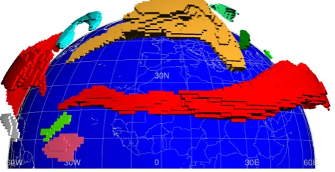
Fig. 1. Example illustration showing all detected three-dimensional features at a single time step of a segmentation of jet streams in the Northern Hemisphere (perspective projection, vertically exag-gerated). Different colors indicate different features.
Our algorithm outputs the information obtained during feature tracking in form of an event graph, a directed acyclic graph (cf. Samtaney et al., 1994; Reinders, 2001). The set of nodes of the event graph corresponds to the set of all detected 3-D-features. If a connection between two 3-D-features of two consecutive time steps is detected within the feature tracking step, this connection is represented as an edge in our graph. The formal definition of the event graph is as follows:
Definition 4 (Event graph) The graphG:=(F,E), where
F is the set of all detected features andE⊆ {(a,b)|a∈Ft; b∈Ft+1;t=1,...,tmax−1}is the set of all edges represent-ing a direct connection between features of two consecutive time steps, is called event graph.
Note that there are several ways to define what “direct connection between features of two consecutive time steps” means. We discussed several different feature tracking ap-proaches in Sect. 1.2, and discuss the details of the methods used by our algorithm in Sect. 3.2.
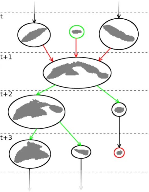
Our final four-dimensional segments, each representing one atmospheric phenomenon and its development over time, are already contained in the event graphGas the connected sets of 3-D-features (see schematic example in Fig. 2). Such distinct sets of connected nodes of a graph, together with the connecting edges, are called connected components. Definition 5 (Segment) Let GS=(S,ES) denote a con-nected component of G. ThenS is called a segment, rep-resenting all features associated with one atmospheric phe-nomenon as it develops over time andGSis called the event graph ofS containing all edgesESbetween connected fea-tures ofS.
Fig. 2. Part of an example event graph of a single 4-D-segment. Nodes are depicted by ellipses including shapes of the correspond-ing 3-D-features. Connectcorrespond-ing edges are depicted by arrows, dashed lines indicate the border between features of different time steps. The green ellipse indicates a genesis event, and the red ellipse a lysis event.
The events can be detected through an inspection of the con-necting edgesESofGSin the following way:
– A genesis event is detected if a node in the event graph has no incoming edges. For example, there is a genesis event at the node depicted by the green ellipse in Fig. 2. – A lysis event is registered at nodes without outgoing
edges. See the red ellipse in Fig. 2 for an example. – If a node has more than one incoming edge, we register
a merging event. This is the case at the node with the red incoming edges in Fig. 2.
– A splitting event exists at nodes with multiple outgoing edges. All nodes with green outgoing edges in Fig. 2 are associated with a splitting event.
Since features at the first time step have no incoming edges, we cannot tell genesis events, defined the way de-scribed above, apart from situations where a phenomenon
simply enters the sampled data domain. In order to avoid spurious results, we exclude the first time step from the de-tection of our genesis events. We have an analogous situation regarding lysis events at the last time step and we therefore exclude them as well. Note that for some applications it can be reasonable to replace genesis events at the first time step and lysis events at the last time step by entry and exit events, respectively. Reinders (2001) detected entry and exit events as well, but with respect to the spatial, not the tempo-ral boundaries of the observed system.
Our algorithm is capable of estimating the locations of the occurring events not only on a feature but on a per-sample basis. In case of genesis and lysis events, all sam-ples of each single involved feature are associated with the respective event. The detection of the locations of merging and splitting events is more involved, as described in detail in Sect. 3.3. In all cases, we denote the result of these attri-butions as follows.
Definition 6 (Event locations) The localization of the oc-curring events is represented by the set T ⊂ X × {“genesis”,“lysis”,“merging”,“split t ing”}. This set contains all involved samples together with an annotation in-dicating the event types that occur at the respective positions of the samples on the point lattice.
2.3 Feature detection predicates
The way in which our algorithm selects and clusters the samples of the input dataset to create the relevant three-dimensional features depends on the formulation of three dif-ferent predicates. We incorporated ideas from region grow-ing and other segmentation methods that use different types of binary predicates for feature detection. The “selective vi-sualization” method proposed by Van Walsum (1995) uses a selection criterion and a connectivity criterion in order to select and cluster samples from the input dataset. In other methods, a global homogeneity criterion is used for the iden-tification of connected regions of interest, see Zucker (1976), Jain et al. (1995), and Pal and Pal (1993).
Our method selects single samples of our input dataset us-ing a local selection criterion (l). Samples are clustered by means of a local homogeneity criterion (h). A global selec-tion criterion (g) is used to select the final segments at the end of the segmentation process. The main task to be ful-filled before the algorithm can be applied to different types of atmospheric phenomena is to find adequate and applicable predicatesh,landg.
Definition 7 (Local selection criterion) The local selection criterion l:X→ {TRUE,FALSE}decides whether or not a single sample belongs to a potential three-dimensional fea-ture, based on any of its local characteristics.
the formulation of a local criterion may be sufficient for a full classification of the features we want to identify. A sim-ple but nevertheless powerful formulation of such a selection criterion is to test whether the values of the samples lie above or below a given fixed threshold. In our case study on jet streams, for example, we used a height-dependent threshold on the wind speed.
For the clustering of the selected samples, we use a binary predicate called the local homogeneity criterion. We define it as follows:
Definition 8 (Local homogeneity criterion) The local ho-mogeneity criterion h:X×X→ {TRUE,FALSE} decides whether a given pair of neighboring samplesx:=xi,j,k,t∈ X and x0 :=xi+i0,j+j0,k+k0,t+t0 ∈X with i0,j0,k0,t0 ∈
{−1,0,1}; |i0| + |j0| + |k0| + |t0| =1 belongs to the same seg-ment, or not.hhas to be commutative.
For scalar sample values, an obvious formulation of such a predicate could be a threshold on the difference between the sampled values ofx and the adjacent samplex0. If we analyze a vector field, we could impose a threshold on the angle between the directions ofx and x0. In many of our applications, however, we know in advance that our input data field will be homogeneous, such that we may assume
h(x,x0):=TRUEfor all pairs of adjacent samplesx,x0. Many applications based on region growing methods, for example Silver and Zabusky (1993), start the segmentation with sets containing single seed points. Neighboring sample points are added iteratively to these sets, as long as they are still associated with the same features (for example based on thresholding or on a global homogeneity criterion). The ini-tial seed points often correspond to extremal points, such as local minima or maxima, of the underlying data. Since we aim for a segmentation in only one iteration over the dataset, we cannot know in advance whether a connected set of sam-ples will contain any such extremal point or not. To compen-sate this, we use an additional predicate for discarding seg-ments at the end of the iteration based on any of their global attributes. This predicate is the global selection criterion: Definition 9 (Global selection criterion) The global selec-tion criterion g:P(F )→ {TRUE,FALSE}decides whether or not to keep a candidate four-dimensional segment based on any of its global characteristics.
For the segmentations of jet streams, we decided to use the global selection criterion as a filter on the lifespan of the detected wind events. In order to exclude short-lived peaks of wind speed, we decided to discard segments with a lifespan of less than 24 h.
3 Segmentation algorithm
In the previous section, we conceptually defined the input and output of our algorithm, as well as all required predicates
Algorithm 1
Input: The set of sampled atmospheric dataX, the homogeneity criterionh, the local selection criterionland the global selection criteriong. Output: The event graphsGSicontaining all segments S1,...,Sncorresponding to the detected atmospheric phenomena to-gether with the precise event locationsT.
1: F:= ∅;E:= ∅;T:= ∅ FThe sets of all features, connecting edges and event locations
2: c:= ∅ FAn array of all candidate features. 3: fort:=1,...,tmaxdo
4: for eachxi,j,k,twithl(xi,j,k,t)==TRUE do
5: ci,j,k,t:=new candidate feature(xi,j,k,t)
6: for each already visited neighborxi0,j0,k0,t do
7: ifh(xi,j,k,t,xi0,j0,k0,t)==TRUEandci0,j0,k0,t
ex-ists then
8: merge(ci,j,k,t,ci0,j0,k0,t)
9: end if
10: end for
11: ift >1 and∃m:xi,j,k,t−1belongs toFt−1,mthen
12: E:=E∪(Ft−1,m,ci,j,k,t) Fthese edges are later
replaced by real edges
13: end if
14: end for
15: F:=F∪get real features(c,t ) 16: replace candidate edges(E) 17: ift >1 then
18: E:=E∪extended feature tracking(Ft−1,Ft) 19: T:=T∪find event locations(Ft−1,Ft)
20: end if
21: end for
22: return all connected components (Si,ESi) of (F,E) with g(Si)==TRUEandT
for the characterization of the features we want to detect. This is the basis for describing now in detail (and more tech-nically) the implementation of our algorithm, whose general outline is shown in Algorithm 1. In the following subsec-tions, we will investigate in detail the important steps of the algorithm.
3.1 Feature detection
Feature detection is the process of constructing all sets of samples corresponding to the features of interest. Single samples are selected by means of the local selection criterion, and clustered based on the homogeneity criterion. During execution, the algorithm successively adds samples to candi-date features and merges multiple candicandi-date features as soon as a connection is detected.
The algorithm iterates sequentially over all time stepst. At each time stept, the algorithm investigates all samplesXt
starting atx1,1,1,t and traversing the remaining samples by
increasing the first three indices lexicographically. As soon as a samplex:=xi,j,k,t fulfills the local selection criterionl,
For this, we examine the up to three already visited adja-cent samplesxi−1,j,k,t,xi,j−1,k,t, andxi,j,k−1,t. From these
samples we select those which are already associated with a candidate feature and fulfill the homogeneity criterionh. We then merge these candidate features into one.
The algorithm represents the candidate features using a union-find data structure (cf. Knuth, 1997; Cormen et al., 2009). Each candidate feature is stored internally as a tree. The root of each tree is the unique representative of the can-didate feature. Different cancan-didate features are merged by transforming the root of the tree with smaller height into a child node of the root of the other tree. In our implementa-tion, each candidate feature internally stores a list of indices of all samples associated with the corresponding feature, as well as a set of attributes, such as the center of mass and an approximation of the volume. The list of sample indices and the set of attributes are updated each time two candidate fea-tures are merged. To keep the number of nodes low, we add single samples with only one neighboring candidate feature directly to the existing feature instead of adding a new node to the tree. For the sake of simplicity, we omitted the dis-tinction of this additional case in our algorithm outline. The performance of the union and find operations is further im-proved by using path compression. For a direct access to the candidate features associated with each sample, we store the references in a three-dimensional array. At the end of each time step, the set of all remaining candidate features corre-sponds to the set of real featuresFt.
3.2 Feature tracking
The goal of feature tracking is to identify at every time stept
the relations between features of the previous time stepFt−1 and features of the current time step Ft. This corresponds
to a grouping of features belonging to the same instance of an atmospheric phenomenon. There are many possible ap-proaches to achieve this goal, depending primarily on the at-tributes such as shape, size and speed of the objects to track. Relatively big and slow-moving features, with respect to the sampling frequencies of the data domain, such as jet streams, require a different approach than the tracking of, e.g. po-tential vorticity cut-offs, which in comparison are typically smaller and move faster. Different general approaches for feature tracking have been discussed in Sect. 1. For most of our current applications, it is sufficient to track features based on spatial overlaps of the samples that are associated with the features. This approach is valid since the spatial and temporal sample frequencies are generally high enough with respect to the expected size and speed of the features to track (cf. Samtaney et al., 1994). We keep track of the spa-tial overlaps by maintaining a set of candidate edges, which represent connections from the features of the previous time step to the candidate features of the current time step. An edge is added to the set whenever a samplexi,j,k,t is
asso-ciated with a candidate feature and the sample at the same
location of the previous time step, xi,j,k,t−1, is associated with a feature. For a direct lookup of the candidate fea-tures of samples of the previous time step, we use another three-dimensional array. As soon as the final features are known, the replacement of candidate edges by real edges is straightforward. In the algorithm outline, it is denoted as the replace candidate edges(E) function call.
Despite the fact that in our applications so far, the major-ity of continuations could be handled by testing for spatial overlap, we also identified rare cases where a feature was too small and fast moving, compared to the spatial and temporal resolution of the grid, to be tracked by spatial overlaps only. We therefore apply an additional feature tracking step, in-dicated by the extended feature tracking(Ft−1,Ft) function
call in the algorithm outline. In this extended feature track-ing step, we compare attributes (currently centers of mass and volumes) of pairs of unconnected features. If the differ-ences of the attributes are below a fixed threshold, the two features are regarded as an additional continuation. This is similar to the approaches described in Samtaney et al. (1994) and Reinders (2001), but without predicting the future state of attributes by means of extrapolation.
3.3 Event localization
As soon as all connections between the three-dimensional features are established, we are ready to estimate the loca-tions of the occurring events on a per-grid-point basis (in-dicated by the find event locations(Ft−1,Ft) function call in
the algorithm outline). The localization of events allows us to gain important additional insight in the development of atmo-spheric phenomena. As illustrated in Sect. 4 below, one pos-sible application is the calculation of climatologies of events in order to find areas where events are particularly frequent or rare/absent. The number of events in a certain region can be a measure for the stability of the identified features in this re-gion. In some cases specific event locations can be related to particularly interesting atmospheric processes. An example case study where the location of a single jet stream merging event could be associated with the breaking of a Rossby wave will be presented in Sect. 4.1. Previous methods, including those operating on the full set of samples in grid space, for example by Silver and Zabusky (1993) and Muelder and Ma (2009), only detected the existence of events, but not their precise location in grid space.
The localization of the genesis and lysis events is straight-forward: we associate all samples of features without a pre-ceding feature with a genesis event, and all samples of fea-tures without a successive feature with a lysis event. We ex-clude genesis events at the first time step and lysis events at the last time step because we have no information about the history or continuation of these features.
1 1 1
1 1 1 1
1 1 1
1 1
2
2 2 2
2 2
2
1 1 1 1 M M 2 2 2
2 2 2
2 2 2 2
2 2 2
2 2 2
2 2 2
2 2 1 1 1 1 1
1 1 1 1 1
1
1 1
1 1 1
1 1 1 1 1
1 1
M M
M M
M M
M
M
M
1 1 1
1 1 1 1 1
1 1 1 1 1 1
1 1 1 1 1
1 1 1 1
1 1
2 2
2 2 2
2 2 2 2 2
2 2 2 2
2 2 2
2 2
1 1 1
1 1 1 1
1 1 1 1
1 1 1
1 1 1
1 1
1
2 2
2 2
2 2 2
2 2
2 2
2 2
2 M M M M
M M M M
M M M M
M M M M
M M M
M M M
M M M
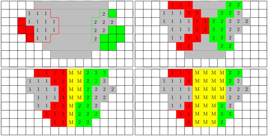
Fig. 3. Two-dimensional example of the applied steps for localizing a merging event. In the top-left picture, gray grid points indicate the location of the merged feature at time stept. Red and green grid points indicate the initial location of the separated features at the previous time stept−1. Grid points with the tag “1” mark the positions where the red and gray features overlap. Grid points with the tag “2” indicate positions where the green and gray features overlap. The pictures to the right and below show the second step of the first growing phase and the final tagging, respectively. Newly tagged regions are depicted in red and green, the positions where both regions touch are indicated by the tag “M” on yellow background. The picture at the bottom-right shows the final state at the end of the second growing phase.
is done analogously by running the procedure in the inverse time direction. The estimation of the position where multi-ple features merge into a new feature is based on a search for grid points that have a similar distance to any two of the single features (this corresponds to grid points lying on the bisectors of the Voronoi regions of the single features). To find these points, we apply a process similar to region grow-ing. We use the sets of grid points of the single features as seed points and let these regions “grow” by tagging all grid points adjacent to the boundaries iteratively. The positions we are interested in are the grid points where these growing regions first touch. Figure 3 provides a two-dimensional il-lustrative example. We limit the growing to the grid points covered by the new feature. Of course, it is very unlikely that the merging occurred exactly at the position of the thin border detected by this growing process. To compensate for this, we enlarge the border into an area allowing for a cer-tain, controllable amount of fuzziness. This enlargement is realized by letting the borders grow for a fixed number of steps in a second growing phase. The choice of the number of steps for this second phase depends on the desired output and on the intended further processing of the event locations. Choosing a greater number of steps leads to a more fuzzy and larger representation of the events.
More formally, the procedure can be described as follows: Assume there is a merging of featuresFt−1,1,...,Ft−1,minto
featureFt,1. At first, we initialize an empty setN in which we will insert elements of the form(i,j,k,n)∈N4. We use these tuples in order to relate certain positions on the point
lattice of our samples, specified by means of indicesi,j,k, to different integer tags n. Initially, for each existing pair of spatially overlapping samples(p,q):=(pi,j,k,t−1,qi,j,k,t)
3.4 Efficiency
In terms of computational efficiency, our method profits from simplifications made on the basis of the prior knowl-edge about the atmospheric features we want to identify and track. Therefore feature identification, tracking, and event localization can be performed within a single iteration over the dataset. Other methods, for example the approach by Muelder and Ma (2009), require at least one iteration over the whole dataset, if all new features and holes in existing features are to be detected. Related approaches, for example Silver and Zabusky (1993), use octrees or other spatial data structures to achieve speedups. Since our algorithm selects, clusters and tracks features during a single iteration over the dataset, there would be no benefit from the additional main-tenance of a spatial data structure. The only exception would be if the available memory was very limited, such that the two additional three-dimensional arrays we use for storing the links to the candidate features of the current time step, and to the features of the previous time step, could not be allocated. In such cases, it would be reasonable to replace these two arrays by an appropriate spatial data structure, in order to save memory at the expense of speed.
4 A climatology of upper-tropospheric jet streams and their events
The new segmentation algorithm has been implemented and tested for different types of atmospheric phenomena. By now, these phenomena were ozone holes, jet streams, cy-clones, and filaments of potential vorticity. In this section we present results from the most extensive of these applica-tions, which was the computation of a two-years climatol-ogy of three-dimensional upper-tropospheric jet streams and their merging and splitting events. Wind fields were taken from the operational ECMWF analyses for the years 2007 and 2008, available every 6 h on 60 vertical levels interpo-lated to a regular longitude/latitude grid with a resolution of 1 degree.
For the detection of upper tropospheric jet streams, we choose the local selection criterion to be a height-dependent wind speed threshold. We accept all samples below 100 hPa (i.e. grid points with pressure larger than 100 hPa) with a hor-izontal wind speed exceeding 40 m s−1. This criterion is mo-tivated by the wind speed threshold criterion used by Koch et al. (2006), who considered jet streams as two-dimensional features of the vertically integrated wind speed between 100 and 400 hPa. Strong winds in the stratosphere, that is at lev-els above 100 hPa, are excluded to focus on jet streams in the upper troposphere. Compared to Koch et al. (2006) we use a 10 m s−1larger threshold, due to the extension of con-sidering jet streams as fully 3-D features instead of 2-D fea-tures of the vertically averaged wind speed. As a side remark, note that recently also Schiemann et al. (2009) and Manney et al. (2011) introduced alternative jet identification schemes,
which focus on the jet axis (i.e. the location in meridional vertical cross-sections where the horizontal wind speed is maximum) and therefore avoided the vertical averaging of the wind speed as performed by Koch et al. (2006). As a global selection criterion, we choose a threshold on the total lifetime of a four-dimensional segment. The idea behind this threshold is to separate real jet stream events from short-lived wind events that exist for less than 24 h. Due to the general homogeneity of the wind speed data from global analyses, we do not state any explicit homogeneity criterion.
Before presenting the climatological results, we start with a brief case study of an interesting episode of Rossby wave breaking and an associated jet stream merging event over the North Atlantic. The aim of this case study is to illustrate the relevance of such jet merging events for atmospheric dynam-ics.
4.1 A Rossby wave breaking event over the North Atlantic
A prominent chain of events including rapid cyclogenesis, an intense warm conveyor belt, the formation of a blocking anticyclone, a subsequent Rossby wave breaking, and even-tually a jet stream merging event occurred during the time pe-riod 20–23 January 2007 over the North Atlantic. Isentropic charts of potential vorticity (PV) on 315 K at 12:00 UTC 20 January reveal a prominent trough with stratospheric PV (i.e. more than 2 pvu) over Eastern Canada and an equally promi-nent ridge with tropospheric PV (i.e. less than 2 pvu) down-stream, over the Western North Atlantic (Fig. 4a). Rapid sur-face cyclogenesis occurred during the previous day beneath the upper-level trough leading to a mature cyclone with a core pressure of less than 970 hPa situated over the Gulf of St. Lawrence. Trajectory calculations (not shown) indicate that the rapid cyclone evolution was associated with a prominent warm conveyor belt (Browning, 1990; Wernli and Davies, 1997), which ascends from the cyclone’s warm sector almost to the 310-K isentrope and enlarges the upper level ridge dur-ing the followdur-ing day (Fig. 4b). In parallel, the trough over the Western North Atlantic elongates into a filamentary “PV streamer” (Appenzeller and Davies, 1992) and a downstream trough evolves to the west of Europe. In between, the upper-level ridge develops into a persistent atmospheric blocking. At this time intense jet streams are present on 315 K (black contours) along both flanks of the PV streamer and the down-stream trough. On the 350-K isentrope, jets exist over the US east coast, over Central Europe, and over Northern Africa. Whereas the first two of these jets are partially aligned with the jet systems on 315 K, the African jet is shallower and only present on the higher isentrope.
Fig. 4. Isentropic potential vorticity on 315 K (colors, in pvu) and wind speed on 315 K (black contours for 40, 50, and 60 m s−1) and on 350 K (orange contours for 40, 50, and 60 m s−1) at (a) 12:00 UTC, 20 January 2007, (b) 12:00 UTC, 21 January 2007, (c) 18:00 UTC, 22 January 2007, and (d) 00:00 UTC, 23 January 2007. The 2-pvu contour denotes the dynamical tropopause.
curved jet stream to the north of the blocking on 315 K in-tensifies (Fig. 4c). Six hours later, at 00:00 UTC, 23 Jan-uary (Fig. 4d), the downstream trough reaches into the West-ern Mediterranean and its associated jet stream on 315 K be-comes vertically aligned with the northern extension of the African jet on 350 K. A similar event has been described by Martius et al. (2010) (their Fig. 5) who emphasized the importance of such a jet merging event for a kinetic energy transfer from the extratropical to the subtropical waveguide. Recently, Martius and Wernli (2012) corroborated the rele-vance of these extratropical wave breaking events (and asso-ciated jet mergings) for the intensification of the subtropical jet over Africa.
Figure 5 shows the three-dimensional structure of the jet streams associated with the jet stream merging event over Gibraltar between 18:00 UTC, 22 January and 00:00 UTC, 23 January, as identified with the new segmentation algo-rithm. The previously discussed jet streams to the north of the blocking and over Europe, and the elongated sub-tropical jet reaching from Northern Africa to the Western North Pacific are clearly visible. The red region in the second panel highlights the merging of the extratropical and subtropical jets, as discussed above. This brief case study illustrates that jet merging events can be associated with prominent events of extratropical Rossby wave break-ing and an associated momentum transfer from a midlati-tude to a subtropical jet stream. According to climatolo-gies of Rossby wave breakings (e.g. Wernli and Sprenger,
2007) such events are most likely to occur over the Eastern North Atlantic/Western Mediterranean and Eastern North Pa-cific/Western North America. It will be therefore interesting to consider the climatological occurrence of jet streams and their merging (and splitting) events in the following subsec-tions.
4.2 Frequency of jets, jet merging, and jet splitting
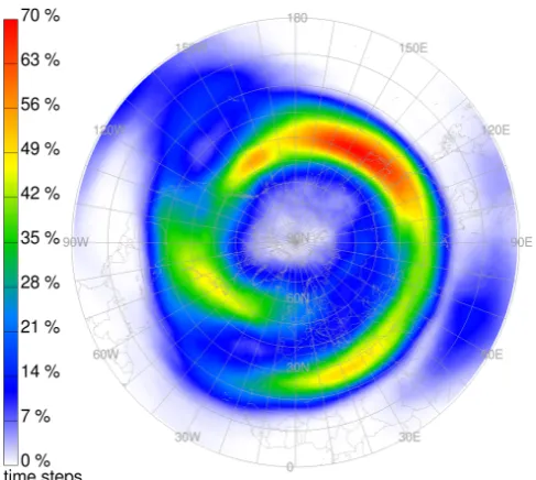
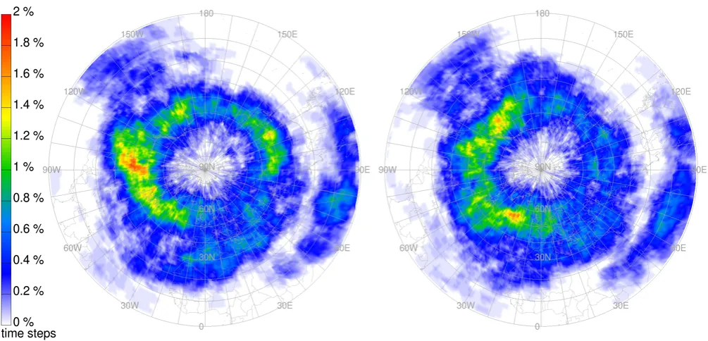
With the results of the segmentation, we are able to compile a climatology of the frequency of jet streams and their gene-sis, lygene-sis, merging, and splitting events. Figure 6 depicts the spatial distribution of all detected jet streams during the two-year time period. In order to obtain a two-dimensional plot, we calculated the jet stream frequency at each horizontal po-sition as the ratio between the number of time steps at which a jet stream was detected at any observed vertical level (i.e. levels below 100 hPa), and the total number of time steps.
Our results agree favorably with the previous climatol-ogy by Koch et al. (2006), despite the different time peri-ods (2007–2008 vs. 1979–1993) and the slightly different jet stream definition. The overall frequency maximum is located over Japan (with values exceeding 70 %) and secondary max-ima are located over Newfoundland and Libya/Egypt. The general spiral-like shape of the region with high jet stream frequencies is also well reproduced, corroborating the relia-bility of the new approach.
Fig. 5. Two successive time steps of a jet stream segmentation at 18:00 UTC, 22 January 2007 (left) and 00:00 UTC, 23 January 2007 (right). The red highlighted region in the panel on the right indicates the location of a merging event. At the previous time step (see panel on the left) the two jet stream features were still separated. All non-event samples are shaded according to the wind speeds at their respective positions.
Fig. 6. Two-year climatology of the spatial distribution of jets iden-tified with the new segmentation method. Values indicate the fre-quency of jet stream occurrences (in %).
merging and splitting events, as shown in Fig. 7. These pat-terns are obviously very different from the overall jet stream frequency distribution. Clear maxima of both mergings and splittings occur in the Western Northern Hemisphere, in
particular over North America. Secondary maxima are found to the north of the Tibetan Plateau and over North Africa. This indicates on the one hand that the very high jet stream frequency over the Western North Pacific is associated with very stable jets that experience comparatively little merging and splitting events. On the other hand the much higher fre-quency of these events in regions mentioned above is qual-itatively consistent with a high frequency of Rossby wave breaking (Wernli and Sprenger, 2007). Future studies will be required to better understand the global linkage between wave breaking and jet stream merging and splitting events.
4.3 Lifetime and stability of jet segments
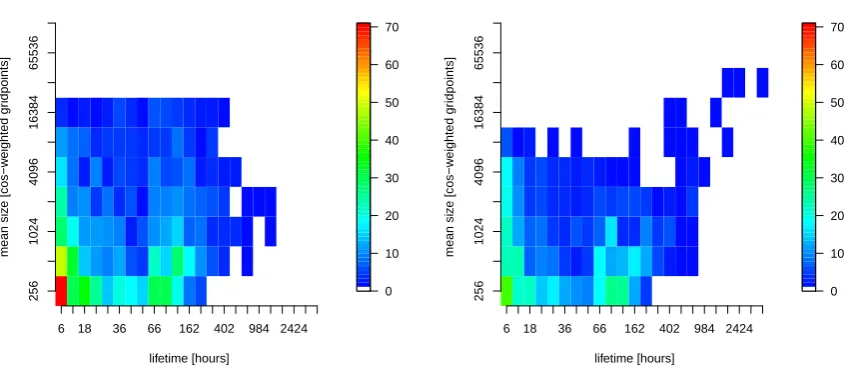
The climatology indicates that jet merging and splitting is particularly frequent in one half of the Northern Hemisphere (from approximately 120◦W to 60◦E). We call this region the “North Atlantic region”, in contrast to the “North Pacific region” where the identified jet stream segments appear to be more persistent. In order to get statistical evidence for the differences in the stability of these segments in the two semi-hemispheres, we further investigate the size and lifetime of these jet segments.
Fig. 7. Two-year climatology of the spatial distribution of (left) jet stream merging and (right) jet stream splitting events. Values indicate the event frequencies (in %).
very stable, long-lived and maybe quasi-stationary jet stream segments, and highly transient segments that break apart and re-merge at frequent intervals. In order to achieve this goal, it is useful to introduce sub-segments.
A sub-segment is a subset of a 4-D segment without any major merging and splitting event. The decision whether or not a connection between two 3-D features of a segment is considered a connection between nodes of the same sub-segment is taken as follows: For each featureFt,i, we pick
the successorFt+1,j whose size is closest to the size ofFt,i
(if present). If now out of all ofFt+1,j’s predecessorsFt,i
is the one with the closest size toFt+1,j, we register a valid
sub-segment continuation between these two features. Out of these sub-segment continuations we are able to construct the complete sub-segments of each 4-D segment.
Additionally, for every sub-segment, we compute its aver-age center of mass, size and lifetime and use this information to attribute the sub-segments to either the North Atlantic or the North Pacific region. The size of the sub-segments is ap-proximated by the number of respective grid points, weighted with the cosine of the latitude of the corresponding position. Figure 8 shows the statistical results of this analysis for the two semi-hemispheres. There are many relatively small and short-lived segments in both regions. Large segments are less frequent. Very large segments, which contain about 15 000 grid points or more, have a lifetime of only up to 400 h in the North Atlantic. In contrast, segments of this size (or larger) all have a lifetime of about 400–3500 h in the North Pacific. Clearly, these huge and long-lived segments dominate the
jet stream pattern in the North Pacific area and contribute essentially to the maximum jet stream frequency in this re-gion. This finding is also consistent with the previously dis-cussed results on the frequency of jet stream splitting and merging events over the North Atlantic and North Pacific, respectively.
5 Conclusions
We presented a new segmentation method with per-grid-point localization of merging and splitting events. The method is capable of efficiently detecting three-dimensional atmospheric features and their development over time. We adopted ideas from several methods from the field of flow visualizations, as described in Sect. 1. However, our method is unique in that it is capable of estimating the locations of merging and splitting events in grid space. In addition, we could simplify the implementation to the point that we only need a single iteration over the dataset. By selecting and clus-tering the data during this iteration, we avoid the construction of additional spatial data structures, as for example done by Silver and Zabusky (1993). Muelder and Ma (2009) track single features very efficiently by operating on the bound-ary of the feature only. However, if new features (or holes inside existing features) should be detected, a full iteration over the dataset (except for the already detected boundaries) is unavoidable.
Sub−segments Atlantic region
lifetime [hours]
mean siz
e [cos−w
eighted gr
idpoints]
6 18 36 66 162 402 984 2424
256
1024
4096
16384
65536
0 10 20 30 40 50 60 70
Sub−segments Pacific region
lifetime [hours]
mean siz
e [cos−w
eighted gr
idpoints]
6 18 36 66 162 402 984 2424
256
1024
4096
16384
65536
0 10 20 30 40 50 60 70
Fig. 8. Histograms relating the size to the lifetime of jet stream sub-segments in the North Atlantic (left) and North Pacific (right) region, respectively. The colors represent the number of sub-segments of the years 2007 and 2008. The size of each sub-segment is approximated by the sum of the cosines of the latitudes of the corresponding grid points.
applied our method to analyze upper-tropospheric jet streams in the Northern Hemisphere and their stability in different re-gions. So far, the analysis of jet streams was the most exten-sive application of our algorithm. However, first experiments with other atmospheric features, such as ozone holes, cy-clones, and potential vorticity filaments also yielded promis-ing results. Currently, we are workpromis-ing on the identification of cyclones. In contrast to existing methods operating on 2-D fields (e.g. Raible et al., 2008 and studies mentioned in the introduction) we plan to detect and track the cyclones as full 3-D objects. For the detection of 3-D cyclones it may be helpful to perform an analysis of the topology of the un-derlying 3-D wind field, similar to the methods of Mahrous et al. (2004). Fuchs et al. (2008) proposed a different method for performing combined extraction and tracking of vortices from time-dependent flow data.
Some of the objects we plan to address in the future are smaller and faster moving than the jet streams, although the sampling rate of the input data remains comparable. This requires some future improvements of our feature tracking method. We could focus on more involved techniques that make use of the features’ attributes, as proposed for example by Reinders (2001), or on prediction-correction methods as used by Muelder and Ma (2009). Another possible approach is to apply an additional dilation of the samples after feature detection, as proposed by Van Walsum (1995). This dilation of selected samples could possibly be refined by taking into account additional knowledge about the expected direction of movement of the features. The localization of the merg-ing and splittmerg-ing events for non-overlappmerg-ing features is an additional issue which has to be addressed. If we are able to use dilated features for tracking, the event localization could work on the same set of dilated features.
So far our experience with the new segmentation method in terms of computational costs is very positive. The analy-sis of the 2-yr wind field dataset used in this study was per-formed in about five hours on a standard Linux PC. Due to the simple structure of the algorithm consisting mainly of one iteration over the dataset, and due to the way the input data is accessed, the algorithm seems well suited for a future extension towards parallel processing. All this indicates that the method is also capable of analyzing very large datasets, for instance output of long-term climate simulations and/or from ensemble simulations. This will offer novel pathways for an in-depth analysis of flow features in very large climate datasets.
Acknowledgements. We would like to thank Patrick J¨ockel from the DLR (Deutsches Zentrum f¨ur Luft- und Raumfahrt) for his help at the initial stage of this work, and for his introduction to and help-ful suggestions on the topic of ozone hole detection. We are also very grateful for the very detailed and constructive comments from two anonymous referees, which helped to improve the presentation of our algorithm. This project has been funded by the Center for Computational Sciences in Mainz, http://www.csm.uni-mainz.de.
Edited by: H. Garny
References
Appenzeller, C. and Davies, H. C.: Structure of stratospheric intru-sions into the troposphere, Nature, 358, 570–572, 1992. Bauer, D. and Peikert, R.: Vortex tracking in scale-space, in:
Browning, K. A.: Organization of clouds and precipitation in extra-tropical cyclones, in: Extraextra-tropical Cyclones, edited by: Newton, C. and Holopainen, E., Vol. The Erik H. Palmen Memorial Vol-ume, Amer. Meteor. Soc., Boston, 129–153, 1990.
Cormen, T. H., Leiserson, C. E., Rivest, R. L., and Stein, C.: Intro-duction to Algorithms, The MIT Press, 3rd Edn., 568–572, 2009. Fuchs, R., Peikert, R., Hauser, H., Sadlo, F., and Muigg, P.: Par-allel Vectors Criteria for Unsteady Flow Vortices, Visualization and Computer Graphics, IEEE Transactions on, 14, 615–626, doi:10.1109/TVCG.2007.70633, 2008.
Jain, R., Kasturi, R., and Schunck, B. G.: Machine Vision, McGraw-Hill, New York, 1995.
Ji, G., Shen, H.-W., and Wenger, R.: Volume tracking using higher dimensional isosurfacing, in: Visualization, 2003, VIS 2003, IEEE, 209–216, doi:10.1109/VISUAL.2003.1250374, 2003. Knuth, D. E.: The Art of Computer Programming, Volume 1:
Fun-damental Algorithms (3rd Edn.), chap. 2.3.3, 354–355, Addison-Wesley Professional, 1997.
Koch, P., Wernli, H., and Davies, H.: An event-based jet-stream climatology and typology, Int. J. Climatol., 26, 283–301, 2006. K¨onig, W., Sausen, R., and Sielmann, F.: Objective identification of
cyclones in GCM simulations, J. Climate, 6, 2217–2231, 1993. Lambert, S. J.: A cyclone climatology of the Canadian Climate
Centre general circulation model, J. Climate, 1, 109–115, 1988. Limbach, S., Marto, M., J¨ockel, P., Sch¨omer, E., and Wernli, H.:
Die Analyse atmosp¨arischer Str¨omungen, Natur & Geist - Das Forschungsmagazin der Johannes Gutenberg-Universit¨at Mainz, 2, 22–25, 2009.
Mahrous, K., Bennett, J., Scheuermann, G., Hamann, B., and Joy, K.: Topological segmentation of three-dimensional vector fields, IEEE Trans. Visual. Comput. Graph., 10, 198–205, 2004. Manney, G. L., Hegglin, M. I., Daffer, W. H., Santee, M. L., Ray,
E. A., Pawson, S., Schwartz, M. J., Boone, C. D., Froidevaux, L., Livesey, N. J., Read, W. G., and Walker, K. A.: Jet charac-terization in the upper troposphere/lower stratosphere (UTLS): applications to climatology and transport studies, Atmos. Chem. Phys., 11, 6115–6137, doi:10.5194/acp-11-6115-2011, 2011. Martius, O. and Wernli, H.: A trajectory based investigation of
physical and dynamical processes that govern the temporal evo-lution of the subtropical jet streams over Africa, J. Atmos. Sci., in press, 2012.
Martius, O., Schwierz, C., and Davies, H. C.: Tropopause-level waveguides, J. Atmos. Sci., 67, 866–879, 2010.
Muelder, C. and Ma, K.-L.: Interactive feature extraction and tracking by utilizing region coherency, in: Visualiza-tion Symposium, 2009. PacificVis ’09. IEEE Pacific, 17–24, doi:10.1109/PACIFICVIS.2009.4906833, 2009.
Murray, R. J. and Simmonds, I.: A numerical scheme for tracking cyclone centres from digital data, Part I: development and oper-ation of the scheme, Aust. Meteorol. Mag., 39, 155–166, 1991. Pal, N. R. and Pal, S. K.: A review on image segmentation
tech-niques, Pattern Recognition, 26, 1277–1294, doi:10.1016/0031-3203(93)90135-J, 1993.
Post, F. H., Vrolijk, B., Hauser, H., Laramee, R. S., and Doleisch, H.: The State of the Art in Flow Visualisation: Feature Extraction and Tracking, Comput. Graph. Forum, 22, 775–792, 2003. Raible, C. C., Della-Marta, P. M., Schwierz, C., Wernli, H., and
Blender, R.: Northern hemisphere extratropical cyclones: a com-parison of detection and tracking methods and different reanaly-ses, Mon. Weather Rev., 136, 880–897, 2008.
Reinders, F.: Feature-based visualization of time-dependent data, Ph.D. thesis, University of Delft, 2001.
Samtaney, R., Silver, D., Zabusky, N., and Cao, J.: Visualiz-ing features and trackVisualiz-ing their evolution, Computer, 27, 20–27, doi:10.1109/2.299407, 1994.
Schiemann, R., L¨uthi, D., and Sch¨ar, C.: Seasonality and interan-nual variability of the westerly jet in the Tibetan plateau region, J. Climate, 22, 2940–2957, 2009.
Siegesmund, M.: Visuell gest¨utzte Mustererkennung zur Identifika-tion und KlassifikaIdentifika-tion von Ozonl¨ochern, Master’s thesis, Uni-versit¨at Rostock, 2006.
Silver, D. and Wang, X.: Tracking and visualizing turbulent 3D features, Visualization and Computer Graphics, IEEE Trans-actions on Visualization and Computer Graphics, 3, 129–141, doi:10.1109/2945.597796, 1997.
Silver, D. and Wang, X.: Visualizing evolving scalar phe-nomena, Future Generation Computer Systems, 15, 99–108, doi:10.1016/S0167-739X(98)00048-X, 1999.
Silver, D. and Zabusky, N.: Quantifying Visualizations for Re-duced Modeling in Nonlinear Science: Extracting Structures from Data Sets, J. Vis. Commun. Image Re.n, 4, 46–61, doi:10.1006/jvci.1993.1005, 1993.
Ulbrich, U., Leckebusch, G. C., and Pinto, J. G.: Extra-tropical cyclones in the present and future climate: a review, Theor. Appl. Climatol., 96, 117–131, 2009.
Van Walsum, T.: Selective visualization on curvilinear grids, Ph.D. thesis, Delft University of Technology, 1995.
Weigle, C. and Banks, D.: Extracting iso-valued features in 4-dimensional scalar fields, in: Volume Visualization, 1998, IEEE Symposium on Volume Visualization, 103–110, doi:10.1109/SVV.1998.729591, 1998.
Wernli, H. and Davies, H. C.: A Lagrangian-based analysis of ex-tratropical cyclones, I, The method and some applications, Quart. J. Roy. Meteor. Soc., 123, 467–489, 1997.
Wernli, H. and Schwierz, C.: Surface cyclones in the ERA-40 dataset (1958–2001), Part I: Novel identification method and global climatology, J. Atmos. Sci., 63, 2486–2507, 2006. Wernli, H. and Sprenger, M.: Identification and ERA15 climatology
of potential vorticity streamers and cut-offs near the extratropical tropopause, J. Atmos. Sci., 64, 1569–1586, 2007.
Wilhelms, J. and Van Gelder, A.: Octrees for faster iso-surface generation, ACM Trans. Graph., 11, 201–227, doi:10.1145/130881.130882, 1992.