© Universiti Tun Hussein Onn Malaysia Publisher’s Office
IJIE
Journal homepage: http://penerbit.uthm.edu.my/ojs/index.php/ijie
The International
Journal of
Integrated
Engineering
NARMAX Model Identification Using Multi-Objective
Optimization Differential Evolution
Mohd Zakimi Zakaria
1,*, Zakwan Mansor
1, Azuwir Mohd Nor
1, Mohd Sazli
Saad
1, Mohamad Ezral Baharudin
1, Robiah Ahmad
21School of Manufacturing Engineering Universiti Malaysia Perlis,
Pauh Putra Main Campus, 02600 Arau, Perlis, Malaysia.
2UTM Razak School of Engineering and Advanced Technology,
Universiti Teknologi Malaysia, Jalan Sultan Yahya Petra, 51400 W. P Kuala Lumpur, Malaysia
*Corresponding Author
DOI: https://doi.org/10.30880/ijie.2018.10.07.018
Received 4 August 2018; Accepted 25 November 2018; Available online 30 November 2018
1. Introduction
System identification is the process of developing a mathematical model of a dynamic system based on measured input-output data. The main purposes of developing mathematical models are for prediction of the behavior of a system and for controller design. This is important in order to improve the efficiency and the effectiveness of the system. There are four procedures that are involved in developing a model of a dynamical system based on observed input-output data. They are acquisition of data, selection of model presentation, parameter estimation, and model validation (Ljung, 1999). Leontaritis & Billings (1985) introduced the nonlinear auto-regressive moving average with exogenous input (NARMAX) model as a representation for a wide class of nonlinear systems. The essence of the NARMAX model is that past outputs are included in the expansions. This makes the model identification easier since fewer terms are required to represent a system. However, it also means that noise in the output must be taken into account when estimating the model coefficients (Billings, 2013). Recently, polynomial NARMAX model has been widely used in nonlinear system identifications such as in control systems (Guo, Wang, & Wang, 2008), power generations (Boaghe, Billings, Li, Fleming, & Liu, 2002; Evans et al., 2001), robotics (Akanyeti, Rañó, & Billings, 2010; Gardiner, Coleman, McGinnity, & He,
Abstract: Multi-objective optimization differential evolution (MOODE) algorithm has demonstrated to be an effective algorithm for selecting the structure of nonlinear auto-regressive with exogeneous input (NARX) model in dynamic system modeling. This paper presents the expansion of the MOODE algorithm to obtain an adequate and parsimonious nonlinear auto-regressive moving average with exogenous input (NARMAX) model. A simple methodology for developing the MOODE-NARMAX model is proposed. Two objective functions were considered in the algorithm for optimization; minimizing the number of term of a model structure and minimizing the mean square error between actual and predicted outputs. Two simulated systems and two real systems data were considered for testing the effectiveness of the algorithm. Model validity tests were applied to the set of solutions called the Pareto-optimal set that was generated from the MOODE algorithm in order to select an optimal model. The results show that the MOODE-NARMAX algorithm is able to correctly identify the simulated examples and adequately model real data structures.
2012) and chemical processes (Aggoune, Chetouani, & Raïssi, 2016; Bucolo, Fortuna, Nelke, Rizzo, & Sciacca, 2002; Fernández et al., 2014). The main advantage of the NARMAX model over alternative models such as the Volterra series is the potential reduction in the number of model terms. For instance, systems that incorporate an output nonlinearity may require an expansion of many hundreds of Volterra kernels while the NARMAX model can produce a compact descriptions for the same systems (Chen & Billings, 1989).
The most challenging problem in system identification is to represent a dynamic system with an adequate and parsimonious model (Sjöberg et al., 1995). In order to obtain a parsimonious structure, the selection of model terms must be included as a part of the identification procedure (Haber & Unbehauen, 1990). In the process of selecting the model terms, several conflicting objectives need to be achieved simultaneously to provide an optimal model structure, i.e. minimization of mean square error of the model prediction and model complexity. Those conflicting objectives are called multi-objective optimization problems (MOPs). A variety of mathematical programming techniques currently exist to solve them, but MOPs from real-world engineering are too complex to solve using conventional optimization methods (Hu, Yang, Sun, Wei, & Zhao, 2017). For solving these problems, evolutionary algorithm (EA) has been introduced. EA can be defined as a stochastic technique inspired by the “survival of the fittest” principle from the evolutionary theory of Darwin and has been used in a wide variety of discipline in optimization technique (Eiben & Smith, 2015). Unlike conventional optimization approaches, EA is suitable for sophisticated optimization problems due to its population-based optimization techniques (Eiben & Smith, 2015).
Since Deb, Pratap, Agarwal, & Meyarivan (2002) introduced elitist non-dominated sorting genetic algorithm (NSGA-II) which is an algorithm based on multi-objective evolutionary algorithm (MOEA), many reported works have applied this algorithm for model structure selection in system identification (Loghmanian, Ahmad, & Jamaluddin, 2009; Loghmanian, Jamaluddin, Ahmad, Yusof, & Khalid, 2012). Zakaria, Mohd Nor, Jamaluddin, & Ahmad (2014) proposed a model structure selection algorithm named Multi-objective optimization differential evolution (MOODE) which is the integration of differential evolution (DE) instead of genetic algorithm (GA) into NSGA-II procedure. The MOODE focuses on two objective functions for model structure selection which are minimizing the error between the proposed model and measured output of the process and minimizing the complexity of the model. For parameter estimation, least square estimation algorithm (LSE) has been used. The comparison of performance between model structure selection algorithm MOODE and NSGA-II that was proposed by Loghmanian et al. (2009) shows that MOODE is better in terms of producing good final solutions, faster convergence and lower computational time (Zakaria, 2013). So far, MOODE has only been employed to detect the structure of nonlinear auto-regressive with exogenous inputs (NARX) model (Zakaria, Mohd Nor, Jamaluddin, & Ahmad, 2014; Zakaria, Saad, Jamaluddin, & Ahmad, 2014).
The aim of the present work is to investigate the performances of MOODE algorithm approach to NARMAX model identification. NARMAX model was chosen because it incorporates past errors as regressors and hence this could make the predicted output from the NARMAX model better (Hornstein & Parlitz, 2002; Mahmoud, 2012). To validate the algorithm, this study starts with the identification of two NARMAX simulated systems with known model structures to show that the algorithm is capable of identifying them effectively. Then, the algorithm was applied on two real experimental data to identify a set of possible solutions called the Pareto-optimal front. Model validity tests were applied in order to select an optimal model from the Pareto-optimal front.
This paper is structured as follows. Section 2 reviews the polynomial nonlinear auto-regressive moving average with exogeneous input (NARMAX) model representation of a system. Section 3 reviews the MOODE algorithm method and model validation process. Section 4 presents and discusses the simulation study by using simulated systems and two real data systems. Finally, the contributions of the study are summarized in Section 5.
2.
NARMAX Model Representation
A NARMAX model can be represented as (Leontaritis & Billings, 1985):
𝑦(𝑡) = 𝐹𝑙(𝑦(𝑡 − 1), … , 𝑦(𝑡 − 𝑛
𝑦), 𝑢(𝑡 − 1), … , 𝑢(𝑡 − 𝑛), 𝑒(𝑡 − 1), … , 𝑒(𝑡 − 𝑛𝑒)) + 𝑒(𝑡) (1)
where ny, nu and ne are the maximum lags for the output, input, and noise terms, respectively, while y(t), u(t) and e(t) are
the output, input and noise signals, respectively. Fl(.) is a polynomial non-linear function with l degree of nonlinearity.
The NARMAX model can be transformed into a linear regression model that can be expressed as:
𝑦(𝑡) = ∑ 𝜃𝑖∅𝑖𝑇(𝑡) + 𝑒(𝑡), 𝑛𝑦≤ 𝑡 ≤ 𝑁 𝑀
𝑖=1
(2)
where θi are unknown coefficients or parameters, ϕi(t) is the regression vector, M is the maximum number of terms of the
regression and N is the size of data. If Equation (2) is written in matrix form, the parameter vector, θ and regression vector, ϕ(t) can be obtained using Equations (3) and (4) respectively:
𝜃𝑇 = [𝜃
∅(𝑡) = [𝑦(𝑡 − 1), … , 𝑦(𝑡 − 𝑛𝑦), 𝑢(𝑡 − 1), … , 𝑢(𝑡 − 𝑛𝑢), 𝑒(𝑡 − 1), … , 𝑒(𝑡 − 𝑛𝑒)] (4)
Referring to Equation (2), the NARMAX model is linear in parameter; hence an algorithm from the least square (LS) family can be used to estimate the parameters, θ. In order to estimate the parameters, θ, the values of noise e(t-1), e(t -2),…,e(t-ne) from Equation (4) must be known. If the noise is known, a simple least square estimation (LSE) or an
ordinary recursive least-square (RLS) algorithm can be used for estimation. However, in general, the noise e(t) is not measurable and the recursive extended least square (RELS) method can be used in order to resolve the problem (Mohamed Vall & M’hiri, 2008). In the RELS algorithm, the sequence of e(t) is estimated iteratively. The RELS procedure can be summarized by the following steps (Aldemir & Hapoglu, 2015):
1. Vector of ϕ(t) is formed using input u(t), output y(t) and the prediction error e(t). The prediction error is calculated using:
(5)
2. The covariance matrix, P(t) is updated using:
(6)
3. The parameter estimation is updated using:
(7)
4. At the next sample, the calculation repeats itself from step 1
The initial values of e(t-1), e(t-2),…,e(t-ne) and parameter vector, θ(t)are set to zero and P(t) is initialized to a very large
identity matrix since no information is available in the beginning.
3.
Modeling Procedures
3.1
Overview of MOODE Algorithm Integrated with NARMAX Model
MOODE algorithm is a model structure selection algorithm inspired by Zakaria et al., (2014) that was based on the integration of differential evolution (DE) into elitist non-dominated sorting genetic algorithm (NSGA-II) procedure but without the DE selection process. Details of the implementation of MOODE for NARMAX model structure selection in modeling dynamic systems are as follows:
Step 1: Model parameter setting. Define model parameters such as the orders of input, output, noise lags and degree of nonlinearity, nu, ny, ne and l. Load an available input-output and noise data set. Recursive extended least square
(RELS) algorithm is applied in this step. RELS algorithm is applied by using the maximum regression vector and the noise terms are collected iteratively. Then, create the regressors of the NARMAX model using the input-output data and estimated noise terms.
Step 2: DE parameter setting. The DE parameters such as population size (NP), crossover rate (CR), mutation rate (MR), lower boundary (L), upper boundary (H) and maximum generation (Gen) are specified except for the value of vector size (D) which is equal to the size of regression vector that has been generated in Step 1.
Step 3: Model representation for initial population. Generate random vectors, so-called chromosomes of the population, within the lower boundary (L) and upper boundary (H).
Step 4: Define two objective functions. Mean square error (MSE) between the proposed model and measured output of the process and model complexity.
Step 5: Produce parent population (Pt) with size NP. For each vector of the population, the values of the objective
functions are evaluated as in Step 4. Based on these objective functions, each vector of the population is ranked and crowding distance of each vector is calculated. Then the vectors of the parent population are sort based on its rank and the value of crowding distance. This rank sorting is according to priority based on the number of rank with rank 1 being is the first, followed by rank 2 and so on. If the ranks of the vectors are within the same rank, sorting is done based on the value of crowding distance.
Step 6: Create new vectors from the parent population. From Step 5, three vectors of the population are chosen randomly, which is evolved to create new vectors through two genetic operators: mutation and crossover. This step repeats until the size of population is achieved.
Step 7: Create offspring population (Qt) with sizeNP. After the new vectors are produced, Step 4 is repeated in order
to evaluate the fitness of the vectors based on the objective functions. The production of offspring population is the same as the parent population in Step 5.
( ) ( ) T( ) ( 1)
e t y t
t t( 1) ( ) ( ) ( 1) ( ) ( 1)
1 ( ) ( 1) ( )
T
T
P t t t P t
P t P t
t P t t
( )t (t 1) P t( ) ( ) ( )t e t
Step 8: Create new generation of population (Pt+1) with sizeNP. The parent population and offspring population are
combined with the size 2NP. Then, Pt+1is obtained by using crowded tournament selection. Step 6 till Step 8 is
repeated until the maximum number of generation (Gen) is reached.
Step 9: Results illustration. The solutions which are the set of possible model structures that can minimize the two objective functions are plotted in a single graph. The set of possible model structures are represented by the points of Pareto-optimal front.
3.2
Model Validation
Model validation is the final procedure in system identification. This is important in order to check whether the model fits the data adequately without any bias. Referring to the overview of the MOODE algorithm, the Pareto-optimal front graph showing the set of possible model structures will be generated. For simulated systems in which the structure and the parameters of the models are known, the final model can be validated directly by comparing the number of exact terms and the estimated parameters (Loghmanian et al., 2009; Zakaria, Jamaluddin, Ahmad, & Loghmanian, 2012). However if the data is from a real system process, model validity test technique needs to be applied in choosing the final model. In this study, two model validity tests are considered; model predicted output (MPO) and correlation tests. The priority in choosing possible model structures from the Pareto-optimal front graph for validation process will be based on the complexity of the models. The models with about 10 significant terms are usually sufficient to capture the dynamic of highly nonlinear system process (Chen, Billings, & Luo, 1989). So, mostly models that have number of terms 10 and below will be selected to go through the model validity tests. The first model validity test used in this study is the MPO test (Billings & Mao, 1998):
𝑦̂𝑀𝑃𝑂 = 𝐹̂(𝑦̂(𝑡 − 1), … , 𝑦̂(𝑡 − 𝑛𝑦), 𝑢(𝑡 − 1), … , 𝑢(𝑡 − 𝑛𝑢)) (8)
where the MPO output is based on the previous predicted output and input data. is the nonlinear function f( . ). MPO is an efficient model assessment because the prediction errors at previous time instances are inherited by the predictions at later time instances making it more sensitive to the unmodelled terms (Billings & Mao, 1998). The estimated standard error of the regression, σ of the model is calculated to further assess the adequacy of the prediction models from the MPO test where:
𝜎
𝑒𝑠𝑡= √
∑(𝑦 − 𝑦̂
𝑁
(9)Another model validation included in this study is correlation tests. The tests are able to indicate the adequacy of the model by plotting graphs of the confidence bands. The confidence bands are estimated as 95% confidence limits that are approximately ±1.96/√𝑁 where N is the data length. The correlation functions (Billings & Voon, 1986b) used in this study are based on the following equations:
∅𝜀𝜀(𝜏) = 𝐸[𝜀(𝑡)𝜀(𝑡 − 𝜏)] = 𝛿(𝑡), ∀𝜏
∅𝑢𝜀(𝜏) = 𝐸[𝑢(𝑡)𝜀(𝑡 + 𝜏)] = 0, ∀𝜏
∅𝑢̅2𝜀(𝜏) = 𝐸[𝑢̅2(𝑡)𝜀(𝑡 + 𝜏)] = 0, ∀𝜏
∅𝑢̅2𝜀2(𝜏) = 𝐸[𝑢̅2(𝑡)𝜀2(𝑡 + 𝜏)] = 0, ∀𝜏
∅(𝑢𝜀)𝜀(𝜏) = 𝐸[𝜀(𝑡)𝑢(𝑡)𝜀(𝑡 + 𝜏 + 1)] = 0, ∀𝜏
(10)
where ϕ, ε(t), u(t) and δ(t) represents the standard correlation function, the residual sequence, and the input of the system respectively with the delta function. E[.] being the expectation operator.
ˆ
4.
Simulation Study
This section demonstrates the MOODE algorithm for NARMAX model identification. The main purpose of the simulation study is to investigate the effectiveness of the algorithm. First, two simulated systems examples of polynomial NARMAX models named as SS1 and SS2 were identified. Then, the MOODE algorithm was applied on two real systems named flexible beam system 1 and flexible beam system 2. MOODE parameters used for all simulated and real systems are given in Table 1.
Table 1 - MOODE parameters setting.
Type of parameter Value setting
Population (NP) 50
Generations (Gen) 100
Crossover Rate (CR) 0.7
Mutation Rate (MR) 0.3
Lower Boundary (L) 0.1
High Boundary (H) 0.4
4.1
Case study 1: SS1
In this first simulation example, the following model is used to generate the simulation data which will be used for identification. This example is taken from Chen et al. (1989):
𝑦(𝑡) = 0.5𝑦(𝑡 − 1) + 𝑢(𝑡 − 2) + 0.1𝑢2(𝑡 − 1) + 0.5𝑒(𝑡 − 1) + 0.2𝑢(𝑡 − 1)𝑒(𝑡 − 2) + 𝑒(𝑡) (11)
where the system input u(t) was an independent sequence of uniform distribution with mean zero and variance 1.0. The system noise e(t) was a Gaussian white sequence with mean zero and variance 0.04. The number of data generated was 500. NARMAX model parameters setting used in this algorithm are the same with the parameters setting from Chen et al. (1989). The parameters set were three input-output lags, three noise terms lags (nu= ny= ne= 3) and two degree of
nonlinearity (l = 2). The maximum number of model terms was 55 and the possible models to be chosen were 255 – 1 which is equivalent to 3.60 × 10¹⁶.
Fig. 1 illustrates the Pareto-optimal front for the SS1 system. The number of solutions in the Pareto-optimal front is supposed to be same as the number of population setting which was 50. However, there are only seven solutions in the Pareto optimal front as shown in Fig. 1. A reason behind this situation is that some solutions were repeated and were therefore counted as single solution which is called repeated solution. To inspect more about these seven solutions and to investigate whether the Pareto optimal front contains the expected solution for SS1 system, the details of the seven solutions obtained are summarized in Table 2.
Fig. 1 - Pareto-optimal front for SS1.
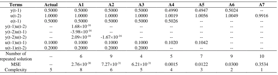
Table 2 - Details of marked models for SS1 system.
Terms Actual A1 A2 A3 A4 A5 A6 A7
y(t-1) 0.5000 0.5000 0.5000 0.5000 0.4990 0.4947 0.5024 --
u(t-2) 1.0000 1.0000 1.0000 1.0000 1.0019 1.0056 1.0049 0.9916
e(t-1) 0.5000 0.5000 0.5000 0.5000 0.5026 -- -- --
y(t-1)u(t-2) -- 1.68×10⁻¹⁶ -- -- -- -- -- --
y(t-2)u(t-1) -- -3.98×10⁻¹⁶ -- -- -- -- -- --
y(t-2)u(t-2) -- 2.09×10⁻¹⁶ -1.67×10⁻¹⁶ -- -- -- -- --
u(t-1)u(t-1) 0.1000 0.1000 0.1000 0.1000 0.1020 0.1042 -- --
u(t-1)e(t-2) 0.2000 0.2000 0.2000 0.2000 -- -- -- --
Number of
repeated solution -- 6 9 4 5 7 9 10
MSE -- 2.76×10⁻³⁰ 7.27×10⁻³¹ 6.21×10⁻³¹ 0.0015 0.0122 0.0300 0.3534
As illustrated in Table 2, the algorithm was able to identify the correct model structures for SS1 system. Model A3 had the exact number of terms and coefficient as the SS1 system. Model A3 also had the lowest MSE value among them which was 6.21×10⁻³¹. Thus, model A3 was chosen as the final model. The number of repeated solution for model A3
was lower compared to others i.e. only 4 which is equivalent to 8% of the population size. This indicates that the number of repeated solution is not important for choosing a final model.
4.2
Case study 2: SS2
The following NARMAX model is used to generate the simulation data which will be used for identification. This example is taken from Billings & Voon (1986a):
𝑦(𝑡) = 0.7578𝑦(𝑡 − 1) + 0.3891𝑢(𝑡 − 1) − 0.03723𝑦2(𝑡 − 1) + 0.3794𝑦(𝑡 − 1)𝑢(𝑡 − 1) + 0.0684𝑢2(𝑡 − 1) + 0.1216𝑦(𝑡 − 1)𝑢2(𝑡 − 1) + 0.0633𝑢3(𝑡 − 1) − 0.739𝑒(𝑡 − 1) − 0.368𝑢(𝑡 − 1)𝑒(𝑡 − 1) + 𝑒(𝑡)
(12)
where the system input u(t) was uniformly distributed with mean 0.2 and the amplitude range was from -0.8 to 1.2. The system noise e(t) was a Gaussian white sequence with mean zero and variance 0.01. The number of data generated was 500. NARMAX model parameters setting used in this algorithm were same with the parameters setting from Billings & Voon (1986a). The parameters set were one input-output lags, one noise terms lags (nu = ny= ne= 1) and three degree of
nonlinearity (l = 3). The maximum number of model terms was 20 and the possible models to be chosen were 220 – 1
which is equivalent to 1.05 × 1006.
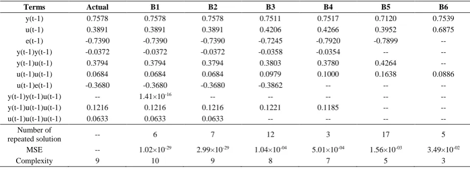
Fig. 2 illustrates the Pareto-optimal front for the SS2 system. As can be seen in Fig. 2, there are six solutions and were marked as B1, B2, B3, B4, B5 and B6. Details of the marked models are given in Table 3. As illustrated in Table 3, model B2 has the exact number of terms and coefficient as the SS2 system. Hence, although model B1 has the lowest MSE value among them which is 1.02×10⁻²⁹, and that there is not much difference in the MSE values of model B1 and
B2., model B2 was chosen as the final model. From the both simulations: SS1 and SS2, the NARMAX-MOODE can trace the exact model structure for representing the simulation systems. From Table 2 and Table 3, the other models showed more parsimonious but insignificant in term of adequacy and fit to represent the dynamic of the systems.
Fig. 2 - Pareto-optimal front for SS2.
Table 3 - Details of marked models for SS2 system.
Terms Actual B1 B2 B3 B4 B5 B6
y(t-1) 0.7578 0.7578 0.7578 0.7511 0.7517 0.7120 0.7539
u(t-1) 0.3891 0.3891 0.3891 0.4206 0.4266 0.3952 0.6875
e(t-1) -0.7390 -0.7390 -0.7390 -0.7245 -0.7920 -0.7899 --
y(t-1)y(t-1) -0.0372 -0.0372 -0.0372 -0.0358 -0.0354 -- --
y(t-1)u(t-1) 0.3794 0.3794 0.3794 0.3803 0.3780 0.4264 --
u(t-1)u(t-1) 0.0684 0.0684 0.0684 0.0979 0.1000 0.1638 0.0886
u(t-1)e(t-1) -0.3680 -0.3680 -0.3680 -0.3862 -- -- --
y(t-1)y(t-1)u(t-1) -- 1.41×10⁻¹⁶ -- -- -- -- --
y(t-1)u(t-1)u(t-1) 0.1216 0.1216 0.1216 0.1221 0.1185 -- --
u(t-1)u(t-1)u(t-1) 0.0633 0.0633 0.0633 -- -- -- --
Number of
repeated solution -- 6 7 12 3 17 5
MSE -- 1.02×10⁻²⁹ 2.99×10⁻²⁹ 1.04×10-04 5.01×10-04 1.56×10-03 3.49×10-02
4.3
Case study 3: Flexible Beam System 1
Flexible Beam system called FB system is based on the input-output data originating from Saad et al. (2015). Fig. 3 shows the schematic diagram of this experimental setup.
Fig. 3 - Schematic diagram of the experimental setup (Saad et al., 2015).
In the FB system, two piezoceramic patches model P-876.A12 DuraAct were attached on the surface of the beam to act as disturbance actuator and control actuator. The properties of the aluminium beam are shown in Table 4 and the properties of piezoceramic patches are listed in Table 5. Two linear power amplifiers that have gains up to 20 and output voltage from -200 V to +200 V which are sufficient to amplify the input signals to actuate the piezoceramic patch were used. National Instruments (NI) data acquisition card was used to acquire analog input from the laser displacement sensor and to send analog output signals to the piezo amplifier. Pseudo random binary sequence (PRBS) signal was used to excite the experimental system which has frequency range from 0 to 98 Hz. To measure the beam displacement, a Sunx laser displacement sensor model ANR-1250 (range: 50 +/-10 mm and resolution: 5 µm) was used. The beam displacement was treated as the output of the FB system. Fig. 4 shows the input-output of the FB system which is the time response excited by the PRBS signal and the frequency response of the flexible beam system excited for a duration of 4 s respectively. There are a total of 1000 data samples collected from the flexible beam test rig. The first 700 samples was used for model identification and the remaining 300 samples was used for model validation. These data were collected by Saad et al. (2015).
Table 4 - Properties and dimensions of the aluminum beam.
Parameter Numerical Values
Length (mm) 500
Width (mm) 50
Thickness (mm) 1.1
Young’s modulus (GPa) 71
Density (Kg/m3) 2700
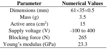
Table 5 - Properties and dimensions of the piezoceramic actuator.
Parameter Numerical Values
Dimensions (mm) 61×35×0.5
Mass (g) 3.5
Active area (cm2) 15
Supply voltage (V) -100 to 400
Blocking force (N) 265
(a) (b)
Fig. 4 - FB system (a) Input (b) Output.
4.3.1
Modeling Flexible Beam System 1 using NARMAX model
NARMAX model parameters setting were four input, output and noise lags (nu = ny= ne= 4) and two degrees of
nonlinearity (l = 2). The maximum number of model terms was 91 and the possible models to be chosen were 291 – 1
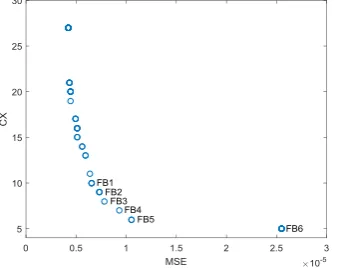
(equivalent to 2.48 × 1027). Fig. 6 illustrates the Pareto optimal front for the FB system. There are 16 possible of model
structure that represents the dynamic behavior of the FB system. The highest model complexity has 27 terms while the lowest has 5 terms. As illustrated in Fig. 5, there are six models selected and they are marked as FB1, FB2, FB3, FB4, FB5 and FB6. These models were selected based on number of terms equal to 10 and below. Details of the marked models are given in Table 6.
Fig. 6 - Pareto-optimal front for FB system.
Table 6 - Details of marked models.
Terms FB1 FB2 FB3 FB4 FB5 FB6
y(t-1) 1.0453 1.0454 1.0428 1.0836 1.0776 1.1344
y(t-3) -0.4296 -0.4443 -0.4651 -0.5113 -0.5192 -04498
u(t-3) 0.0002 0.0002 -- -- -- --
u(t-4) 0.0003 0.0003 0.0003 -- -- --
e(t-2) 0.3522 -- -- -- -- --
e(t-3) 0.3527 0.2978 0.3209 0.3328 0.3360 0.2026
y(t-1)y(t-2) -1.2310 -1.9515 -2.0414 -0.8816 -0.0563 -2.0407
y(t-4)u(t-1) -0.0247 -0.0249 -0.0252 -0.0163 -- --
u(t-1)u(t-4) -0.0001 -0.0001 -0.0001 -0.0001 -4.71×10-05 -3.55×10-05
u(t-2)u(t-2) -0.0003 -0.0003 -0.0003 -0.0003 -0.0003 --
Number of repeated solution
3 3 1 1 2 7
MSE 6.54×10-06 7.33×10-06 7.83×10-06 9.29×10-06 1.05×10-05 2.55×10-05
Complexity 10 9 8 7 6 5
As can be seen in Table 6, models FB4, FB5 and FB6 have large MSE values compared with the others. Although FB1 has the smallest MSE value among the selected models, the difference between FB1, FB2 and FB3 is very small. Thus, the selection for the final model should be done between FB1, FB2 and FB3. These three models will go through the model validity tests i.e. MPO test and correlation test, for choosing an optimal model among them.
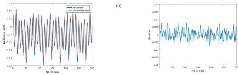
Fig. 7 to Fig. 9 illustrates the MPO test for models FB1, FB2 and FB3. These figures show the output of FB system superimposed on predicted model output and its residual plot. The details of the MSE and R2 values calculated from the
tests for validation set shows that model FB2 has the lowest value compared to others which is 8.84×10-06 for model FB1,
8.36×10-06 for model FB2 and 9.40×10-06 for model FB3.
Based on the estimated standard error of regression, σest for the validation set shows that model FB2 has the lowest
value compared to others which is 0.0029 for model FB2, 0.0030 for model FB1 and 0.0031 for model FB3. Thus, model FB2 produced more accurate prediction output compared to model FB1 and FB3.
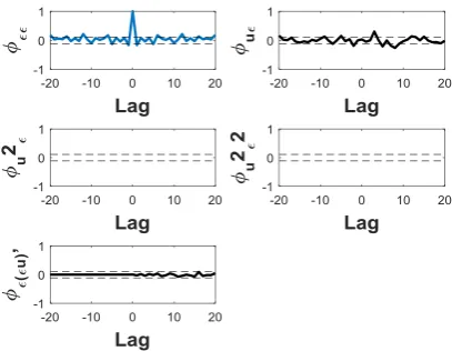
For correlation tests, the illustrations of the plots for the identified models are shown in Fig. 10 to Fig. 12. As illustrated in Fig. 12, model FB3 shows that cross-correlation test, ϕue is not satisfied. This indicates that model FB3 has
correct noise model but the process model is biased (Billings & Voon, 1986b). Meanwhile, model FB1 and FB2 show the correlation tests are well inside the 95% confidence band for each correlation function. Based on all of the model validity tests, model FB2 is suitable to represent the FB system. Model FB2 is given by:
𝑦(𝑡) = 1.0454𝑦(𝑡 − 1) − 0.4443𝑦(𝑡 − 3) + 0.0002𝑢(𝑡 − 3) + 0.0003𝑢(𝑡 − 4) + 0.2978𝑒(𝑡 − 3) − 1.9515𝑦(𝑡 − 1)𝑦(𝑡 − 2) − 0.0249𝑦(𝑡 − 4)𝑢(𝑡 − 1) − 0.0001𝑢(𝑡 − 1)𝑢)𝑡 − 4) − 0.0003𝑢2(𝑡 − 2) = 𝑒(𝑡)
(13)
Table 6 - MSE and R2of MPO tests from the selected models.
Models Estimation Set Validation Set
MSE R2 MSE R2
FB1 1.02×10-05 0.9643 8.84×10-06 0.9667
FB2 1.15×10-05 0.9598 8.36×10-06 0.9685
FB3 1.26×10-05 0.9560 9.40×10-06 0.9646
(a) (b)
Fig. 7 - (a) Model FB1 (a) The output of FB system superimposed on MPO output (b) its residual.
(a) (b)
(a) (b)
Fig. 9 - (a) Model FB3 (a) The output of FB system superimposed on MPO output (b) its residual.
Fig. 10 - Correlation tests for model FB1.
Fig. 12 - Correlation tests for model FB3.
4.4
Case study 4: Flexible Beam System 2
Fig. 13 - Schematic diagram of the experimental setup (Jamid et al., 2017).
To implement the system, an aluminum type cantilever beam of length 450 mm, width 50 mm, and thickness 1.4 mm was considered. Two piezoelectric patches act as disturbance actuator and control actuator were surface bonded to the beam. To measure the beam displacement, a laser displacemnt was used with range 50
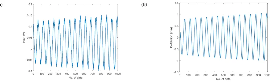
10 mm. Fig. 14 shows the input-output of the system. There are a total of 1000 data samples collected from the experiment where the first 700 samples was used for model identification and the remaining 300 samples was used for model validation. These data were collected by Jamid et al. (2017).(a) (b)
Fig. 14 - Flexible beam system 2 (a) Input (b) Output.
4.4.1
Modeling Flexible Beam System 1 using NARMAX model
NARMAX model parameters setting to represent the system were four input, output and noise lags (nu = ny= ne= 4)
and two degrees of nonlinearity (l = 2). The maximum number of model terms was 91 and the possible models to be chosen were 291 – 1 (equivalent to 2.48 × 1027). Fig. 15 illustrates the Pareto-optimal front for the system. There are 13
possible of model structure that represents the dynamic behavior of the system. The highest model complexity has 22 terms while the lowest has 4 terms. Models with the number of terms equal to 10 and below are selected from the Pareto graph. They were marked as F1, F2, F3, F4, F5, F6 and F7 as illustrated in Fig. 15. Details of the marked models are given in Table 7.
Table 7 - Details of marked models.
Terms F1 F2 F3 F4 F5 F6a F7
y(t-1) 0.6870 0.6897 0.6814 0.6979 0.7116 1.1034 1.9576
y(t-2) 1.1874 1.1842 1.2102 1.1907 1.1835 0.7641 -0.9678
y(t-3) -0.5336 -0.5352 -0.5326 -0.5428 -0.5610 -0.8867 -
y(t-4) -0.3685 -0.3664 -0.3885 -0.3750 -0.3610 - -
u(t-2) 0.1671 0.1661 0.0183 0.0183 - - -
u(t-4) -0.1570 -0.1559 - - - - -
e(t-1) -0.2716 -0.2749 -0.2586 -0.2768 -0.2964 -0.7195 -1.7113
e(t-2) -0.5386 -0.5332 -0.5054 -0.4870 -0.4834 -0.2092 1.3214
y(t-2)e(t-2) 0.0649 - - - -
y(t-3)e(t-4) - - -0.1893 - - - -
y(t-4)e(t-4) -0.1383 -0.1401 - - - - -
Number of repeated
solution 5 3 6 3 3 2 10
MSE 1.54×10-05 1.55×10-05 1.68×10-05 1.76×10-05 1.81×10-05 2.04×10-05 2.39×10-05
Complexity 10 9 8 7 6 5 4
As illustrated in Table 7, models F4, F5, F6 and F7 have large MSE values compared with the models F1, F2 and F3. Model F1 has the smallest MSE value among the selected models however, the difference is very small between models F1, F2 and F3. Thus, the selection for the final model should be done between models F1, F2 and F3. In order to choose an optimal model among them, these three models will go through the model validity tests i.e. MPO test and correlation test.
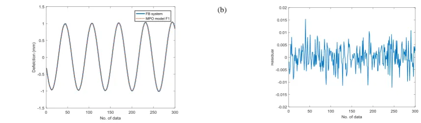
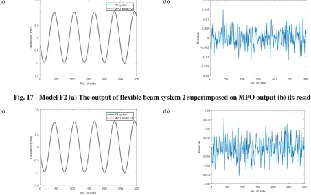
Fig. 16 to Fig. 18 illustrates the MPO test for models F1, F2 and F3. These figures show the output of flexible beam system 2 superimposed on predicted model output and its residual plot. Table 8 illustrates the details of the MSE and estimated standard error of the regression, σest calculated from the MPO output for models F1, F2 and F3. As illustrated
in Table 8, the MSE values from MPO tests for validation set shows that model F2 has the lowest value compared to others which is 1.80×10-05 for model F2, 1.81×10-05 for model F1 and 3.01×10-05 for model F3. Based on the estimated
standard error of regression, σest for the validation set shows that model F2 has the lowest value compared to others which
is 0.0042 for model F2, 0.0043 for model F1 and 0.0055 for model F3. This shows that model F2 produced more accurate prediction output compared to model F1 and F3.
For correlation tests, the illustrations of the plots for the identified models are shown in Fig. 19 to Fig. 21. As illustrated in Fig. 21, model F3 shows that cross-correlation test, ϕee is not satisfied. This incidates that model F3 has the
correct process model but the noise model is incorrect (Billings & Voon, 1986b). Meanwhile, the correlation tests for model F1 and F2 are well inside of the 95% confidence band for each correlation function as shown in Fig.19 and Fig.20. Considering all the model validity tests, model F2 is the best model among the selected models to represent the dynamic of system. Model F2 can be expressed as:
𝑦(𝑡) = 0.6897𝑦(𝑡 − 1) + 1.1842𝑦(𝑡 − 2) − 0.5352𝑦(𝑡 − 3) − 0.3664𝑦(𝑡 − 4) + 0.1661𝑢(𝑡 − 2)
− 0.1559𝑢(𝑡 − 4) − 0.2749𝑒(𝑡 − 1) − 0.5332𝑒(𝑡 − 2) − 0.1401𝑦(𝑡 − 4)𝑒(𝑡 − 4) + 𝑒(𝑡) (14)
(a) (b)
(a) (b)
Fig. 17 - Model F2 (a) The output of flexible beam system 2 superimposed on MPO output (b) its residual.
(a) (b)
Fig. 18 - Model F3 (a) The output of flexible beam system 2 superimposed on MPO output (b) its residual.
Fig. 19 - Correlation tests for model F1.
Fig. 21 - Correlation tests for model F3.
5.
Conclusion
The present study was designed to determine the effect of multi-objective optimization differential evolution (MOODE) approach to NARMAX model. The results showed that the MOODE algorithm provides an efficient way of determining the NARMAX model structure using two objective functions for both simulated and a real system. The both simulation systems: SS1 and SS2, show the ultimate results where the MOODE-NARMAX can find the exact physical structure of the systems. The models A3 and B2 from Tables 2 and 3 were showed the imitate models for simulation systems SS1 and SS2 respectively. It proves the effectiveness of MOODE-NARMAX in finding the correct model structure for the dynamic systems. For real systems results, the final models were chosen to represent the dynamic systems of the flexible beam system 1 and 2 are models FB2 and F2. The physical model for both models can be referred in equations (13) and (14). The final models were selected after through the model validation tests; MPO and correlation tests as discussed in Section 3.2. Beside, results from the model validity tests show both models were adequate and fit to represent the real systems. Furthermore, this paper also demonstrated the methods to choose a final model from the Pareto-optimal front using model validation tests i.e. MPO and correlation test.
Acknowledgement
The authors would like to acknowledge the support from Universiti Malaysia Perlis (UniMAP) and the Fundamental Research Grant Scheme (FRGS) under a grant number of FRGS/1/2016/TK03/UNIMAP/03/8 from the Ministry of Higher Education Malaysia.
References
[1] Aggoune, L., Chetouani, Y., & Raïssi, T. (2016). Fault detection in the distillation column process using Kullback Leibler divergence. ISA Transactions, 63, 394–400.
[2] Akanyeti, O., Rañó, I., & Billings, S. A. (2010). An application of Lyapunov stability analysis to improve the performance of NARMAX models. Robotics and Autonomous Systems, 58, 229–238.
[3] Aldemir, A., & Hapoglu, H. (2015). Comparison of ARMAX Model Identification Results Based on Least Squares Method.
International Journal of Modern Trends in Engineering and Research, 2. Retrieved from http://www.ijmter.com/published-papers/volume-2/issue-10/comparison-of-armax-model-identification-results-based-on-least-square/
[4] Billings, S. A. (2013). Nonlinear System Identification: NARMAX Methods in the Time, Frequency, and Spatio-Temporal Domains. Chichester, UK: John Wiley & Sons, Ltd.
[5] Billings, S. A., & Mao, K. Z. (1998). Model Identification and Assessment Based on Model Predicted Output. Reseach Report no. 714. University of Sheffield, UK: Department of Automatic Control and Systems Engineering.
[6] Billings, S. A., & Voon, W. S. F. (1986a). A prediction-error and stepwise-regression estimation algorithm for non-linear systems. International Journal of Control, 44, 803–822.
[7] Billings, S. A., & Voon, W. S. F. (1986b). Correlation based model validity tests for non-linear models. International Journal of Control, 44, 235–244.
[8] Boaghe, O. M., Billings, S. A., Li, L. M., Fleming, P. J., & Liu, J. (2002). Time and frequency domain identification and analysis of a gas turbine engine. Control Engineering Practice, 10, 1347–1356.
[9] Bucolo, M., Fortuna, L., Nelke, M., Rizzo, A., & Sciacca, T. (2002). Prediction models for the corrosion phenomena in Pulp & Paper plant. Control Engineering Practice, 10, 227–237.
Control, 49, 1013–1032.
[11]Chen, S., Billings, S. A., & Luo, W. (1989). Orthogonal least squares methods and their application to non-linear system identification. INT. J. CONTROL, 50, 1873–1896.
[12]Deb, K., Pratap, A., Agarwal, S., & Meyarivan, T. (2002). A fast and elitist multiobjective genetic algorithm: NSGA-II. IEEE Transactions on Evolutionary Computation, 6, 182–197.
[13]Eiben, A. E., & Smith, J. (2015). From evolutionary computation to the evolution of things. Nature, 521, 476–482.
[14]Evans, C., Fleming, P. J., Hill, D. C., Norton, J. P., Pratt, I., Rees, D., & Rodrı́guez-Vázquez, K. (2001). Application of system
identification techniques to aircraft gas turbine engines. Control Engineering Practice, 9, 135–148.
[15]Fernández, I., Acién, F. G., Berenguel, M., Guzmán, J. L., Andrade, G. A., & Pagano, D. J. (2014). A lumped parameter chemical–physical model for tubular photobioreactors. Chemical Engineering Science, 112, 116–129.
[16]Gardiner, B., Coleman, S. A., McGinnity, T. M., & He, H. (2012). Robot control code generation by task demonstration in a dynamic environment. Robotics and Autonomous Systems, 60, 1508–1519.
[17]Guo, L., Wang, H., & Wang, A. P. (2008). Optimal probability density function control for NARMAX stochastic systems.
Automatica, 44, 1904–1911.
[18]Haber, R., & Unbehauen, H. (1990). Structure identification of nonlinear dynamic systems—A survey on input/output approaches. Automatica, 26, 651–677.
[19]Hornstein, A., & Parlitz, U. (2002). Bias Reduction for Time Series Models Based Support Vector Regression. International Journal of Bifurcation and Chaos,.
[20]Hu, Z., Yang, J., Sun, H., Wei, L., & Zhao, Z. (2017). An improved multi-objective evolutionary algorithm based on environmental and history information. Neurocomputing, 222, 170–182.
[21]Jamid, M. F., Mat darus, I. Z., & Saad, M. S. (2017). Active robust vibration control of a flexible beam. In Proceedings of Mechanical Engineering Research Day 2017 (pp. 450–451).
[22]Leontaritis, I. J., & Billings, S. A. (1985). Input-output parametric models for non-linear systems Part I: deterministic non-linear systems. International Journal of Control, 41, 303–328.
[23]Ljung, L. (1999). System Identification Theory for the User. New Jersey:Prentice-Hall Inc.
[24]Loghmanian, S. M. R., Ahmad, R., & Jamaluddin, H. (2009). Multi-Objective Optimization of NARX Model for System Identification Using Genetic Algorithm. In 2009 First International Conference on Computational Intelligence, Communication Systems and Networks (pp. 196–201). IEEE.
[25]Loghmanian, S. M. R., Jamaluddin, H., Ahmad, R., Yusof, R., & Khalid, M. (2012). Structure optimization of neural network for dynamic system modeling using multi-objective genetic algorithm. Neural Computing and Applications, 21, 1281–1295.
[26]Mahmoud, M. S. (2012). A Comparison of Identification Methods of a Hydraulic Pumping System. IFAC Proceedings Volumes, 45, 662–667.
[27]Mohamed Vall, O. M., & M’hiri, R. (2008). An approach to polynomial NARX/NARMAX systems identification in a closed-loop with variable structure control. International Journal of Automation and Computing, 5, 313–318.
[28]Saad, M. S., Jamaluddin, H., & Darus, I. Z. M. (2015). Active vibration control of a flexible beam using system identification and controller tuning by evolutionary algorithm. Journal of Vibration and Control, 21, 2027–2042.
[29]Sjöberg, J., Zhang, Q., Ljung, L., Benveniste, A., Delyon, B., Glorennec, P.-Y., … Juditsky, A. (1995). Nonlinear black-box modeling in system identification: a unified overview. Automatica, 31, 1691–1724.
[30]Zakaria, M. Z. (2013). Multi-objective model structure optimization using differential evolution for dynamic systems modelling. Universiti Teknologi Malaysia.
[31]Zakaria, M. Z., Jamaluddin, H., Ahmad, R., & Loghmanian, S. M. (2012). Comparison between multi-objective and single-objective optimization for the modeling of dynamic systems. Proceedings of the Institution of Mechanical Engineers. Part I: Journal of Systems and Control Engineering, 226, 994–1005.
[32]Zakaria, M. Z., Mohd Nor, A., Jamaluddin, H., & Ahmad, R. (2014). Multi-Objective Optimization Using Differential Evolution for Modeling Automotive Palm Oil Biodiesel Engine. WSEAS Transaction on Systems and Control, 9, 500–513.