Bayesian Inference for Concomitants based on Weibull Subfamily of Morgenstern Family Under Generalized Order Statistics

(1)

of Morgenstern Family under Generalized Order Statistics

M.M. Mohie EL-Din

Department of Mathematics, Faculty of Science

Al-Azhar University, Cairo, Egypt

[email protected]

Nahed S.A. Ali

Department of Mathematics, Faculty of Education

Ain Shams University, Cairo, Egypt

M.M. Amein

Department of Mathematics, Faculty of Science

Al-Azhar University, Cairo, Egypt

M.S. Mohamed

Department of Mathematics, Faculty of Education

Ain Shams University, Cairo, Egypt

Abstract

In this paper, for Weibull subfamily of Morgenstern family, the joint density of the concomitants of

generalized order statistics

(

GOS

’s) is used to obtain the maximum likelihood estimates (MLE) and

Bayes estimates for the distribution parameters. Applications of these results for concomitants of order

statistics are presented.

Keywords

:

Bayesian estimation, Concomitants, Generalized order statistics, Maximum

likelihood estimation, Morgenstern family.

AMS 2010 Subject Classification:

62F10; 62F15; 62H10; 62H12; 62P99.

1. Introduction

(2)

based on concomitants of generalized order statistics (

GOS

’s). The

pdf

and

cumulative

distribution

function

(

cdf

) of Weibull distribution are given by, respectively:

,

<

0

0,

>

0,

>

,

=

)

1 (





 

y

e

y

f



 y





(1)

,

<

0

0,

>

0,

>

,

1

=

)

(









y

e

y

F

y





(2)

The general theory of concomitants of order statistics has originally studied by David et

al. (1977). Let

(

X

_i

,

Y

_i

)

,

i

=

1,2,



,

n

, be n pairs of independent random variables from

some bivariate population with

cdf

F

(

x

,

y

)

. Let

X

₍_r_:_n₎

be the

r



th

order statistics, then

the

Y

value associated with

X

₍_r_:_n₎

is called the concomitant of the

r



th

order statistics

and is denoted by

Y

_[_r_:_n_]

. Some times exact information are available only on the

concomitants variable since the other variable is only ranked and not measured exactly,

consider for example a group of patients ranked according to the value of their response

to a treatment and subsequently the values of their blood test are observed only on those

patients whose initial value exceeds a threshold, in this situation we have information

only on the concomitants variable. For

1



r

₁

<



<

r

_k



n

, the joint density for

] : [ ] : 1

[r n

,

Y

r_kn

Y



is given by:

,

d

)

,

(

)

|

(

=

)

,

(

=

)

,

(

1 1 ) : , , 1 ( | 1 = 2 1 ] : [ , , ] : 1 [ 1 ] : , , 1 [ k k n k r r i i X Y k i x k x k n k r Y n r Y k n k r r

x

f

x

y

f

y

g

y

g



  





    

(3)

where

(

,

)

=

(

₁

,

)

) : ( , , ) : 1 ( 1 ) : , , 1

( _n k

k r X n r X k n k r

r

x

f

x

f

_



_



. That is, in general, the joint

concomitants of order statistics

_: _] _[ _: _]

1

[r n

,

Y

r_kn

Y



is dependent, where

_, _, _:₎

(

₁

,

)

1

(r r_kn

x

k

f

_



is

the the joint density of

X

(r₁:n)

,



,

X

(r_k:n)

.

The

GOS

’s has introduced by Kamps (1995), the joint density function of the first

r

GOS

’s

X

(1,n,m,k)

,

X

(2,n,m,k)

,



,

X

(r,n,m,k)

,

1



r



n

is given by:

,

...

,

))

(

)(1

))

(

(1

))(

(

=

)

,

(

=

)

,

(

2 1 1 1 1 = 1 = 1 1 ) , , , ( , , ) , , (1, 1 ) , , , , (1,2, r r r X m i X r i i X r i r r k m n r X k m n X r k m n r

x

F

x

F

x

f

c

x

f

x

f





  







_ 

(4)

with parameters

n



N

,

k

>

0

,

m



R

, such that



_r

=

k



(

n



r

)(

m



1)

>

0

,

r _j j r

c

_





1 = 1

=

for all

1



r



n

.

The Morgenstern family discussed by Johnson and Kotz (1975) provides a flexible family

that can be used in such contexts, which is specified by

cdf

and

pdf

, respectively, as

follows:

))],

(

))(1

(

(1

)[1

(

)

(

=

)

,

(

,

x

y

F

x

F

y

F

x

F

y

(3)

1)],

)

(

1)(2

)

(

(2

)[1

(

)

(

=

)

,

(

,

x

y

f

x

f

y



F

x



F

y



f

_X_Y _X _Y



_X _Y

(6)

where



1







1

, and

f

_X

(

x

)

,

f

_Y

(

y

)

, and

F

_X

(

x

)

,

F

_Y

(

y

)

are the marginal

pdf

’s and

cdf

’s of

X

and

Y

respectively. The association parameter



is known as the

dependence parameter of the random variables

X

and

Y

. If



is zero, then

X

and

Y

are independent.

The conditional

pdf

of

Y

given

X

is given by:

1.

1

1)],

)

(

1)(2

)

(

(2

)[1

(

=

)

|

(

|

y

x

f

y





F

x



F

y









f

_Y_X _Y _X _Y

(7)

Mohie El-Din et al. (2015) have proposed the joint density of the concomitants of

GOS

’s

for Morgenstern family, from (3), (4) and (7), the joint density of the first

r

concomitants

of

GOS

’s

Y

[1,n,m,k]

,

Y

[2,n,m,k]

,



,

Y

[r,n,m,k]

,

1



r



n

, for Morgenstern family is given by:

,

1)

)

(

(2

1)

)

(

(2

1)

)

(

1)(2

)

(

1)(2

)

(

(2

1)

)

(

1)(2

)

(

(2

1)

)

(

(2

1

)

(

=

)

,

(

1 = * 1 = 2 1 2 1 1, = , , 2 , 1 1 1, = , , 3 1, = , 2 1 = 1 = 1 ] , , , , [1,2,



















































       i Y r i r i Y r i i i r i i i r r i i i r i i i r k Y j Y i Y ijk r k j i k j i j Y i Y ij r j i j i i Y i r i i Y r i r k m n r

y

F

C

y

F

C

y

F

y

F

y

F

C

y

F

y

F

C

y

F

C

y

f

y

g



   



(8)

where all the constants

C

’s are constant functions of



’s.

In Bayesian approach, the SE loss function which is classified as a symmetric function

and associates equal importance to the losses for overestimation and underestimation of

equal magnitude, many authors study the SE loss in Bayesian inference, see for example,

Calabria and Pulcini (1996), Singh et al. (2002) and Jaheen ((2004a) and (2004b)). The

LINEX loss function which is asymmetric, was first introduced by Varian (1975) and was

widely used by several authors. This function rises approximately exponentially on one

side of zero and approximately linearly on the other side. The GE loss function is also

asymmetric loss function which is used in several papers, for example, Dey et al. (1987),

Dey and Liu (1992) and Soliman ((2005) and (2006)).

In this article, we consider the classical and Bayesian inference of the distribution

parameters for concomitants of

GOS

’s based on two-parameter Weibull subfamily of

Morgenstern family. Approximate Bayesian estimation are obtained under symmetric SE,

asymmetric LINEX and GE loss functions for IP and NIP using Lindley’s approximation

and Markov chain Monte Carlo (MCMC) method. The organization of the paper is as

follows: In Section 2, joint density for concomitants of

GOS

’s based on two-parameter

(4)

estimates of model parameters using Lindley’s approximation and MCMC method are

obtained. Section 3, contains the simulation results and real life data example based on

order statistics as a special case of

GOS

’s. Conclusion is made in Section 4.

2. Classical and Bayesian estimation for concomitants of

GOS

’s

In this section, we study classical estimation such as ML estimation with its approximate

confidence intervals and obtain Bayesian estimation using informative and

non-informative priors under SE, LINEX and GE loss functions for two-parameter Weibull

subfamily of Morgenstern family.

2.1 Maximum Likelihood Estimation

Suppose that

y

=

(

y

₁

,

y

₂

,



,

y

_r

)

is a concomitants of

GOS

’s sample. From (1), (2) and

(8), the log-likelihood function for Weibull subfamily of Morgenstern family is given by:

.

)

2

(1

)

2

(1

)

2

)(1

2

(1

)

2

(1

1

log

=

)

|

,

(

log

=

)

|

,

(

1 = *

1 = 2 1 2 1 1, = , , 2 , 1 1 1, = , 2

1 =

1 1 = 1 =





































 

  

 









 

  

 

  

 

















i y r

i r

i y r

i

i i r i i i r

r i i i r i i i r

j y i

y ij

r

j i j i

i y i

r

i

i r

i i r

i

e

C

e

C

e

C

e

C

y

r

y

L

y

 





(9)

To derive the ML estimation of the unknown parameters



, say



ˆ

_ML

, and



, say



ˆ

_ML

,

we differentiate (9) twice with respect to



and



and then solve the following

non-linear equation numerically by using Newton-Raphson method.

2.2 Bayesian estimation

If we have enough information about the parameter we should use informative prior (IP),

otherwise it is better to consider non-informative prior (NIP). In this section, we want to

obtain Bayesian estimation of the model parameters



,



. Unfortunately, in many cases

the Bayesian estimation can’t be expressed in explicit forms. So, approximate Bayesian

estimation are obtained under IP and NIP using Lindley’s approximation and Markov

chain Monte Carlo (MCMC) method.

2.2.1 Non-informative prior

For Weibull subfamily of Morgenstern family, suppose that



and



are independent

and each of them have the Jeffreys vague prior, respectively:

0

>

,

1

)

(



(5)

0,

>

,

1

)

(







then, the joint NIP of the parameters is given by

0.

>

,

1

)

,

(

1















(10)

The joint posterior density function of the parameters



and



can be written from (1),

(2), (8) and (10) as follow:

,

)

,

(

)

|

,

(

)

|

,

(

* 1 1 = 1 = 1 1 1 * 1

Q

y

e

y

L

y

i r i i y r i r r    







  





















(11)

where

)].

2

(1

)

2

(1

)

2

)(1

2

(1

)

2

(1

1

=

1 = * 1 = 2 1 2 1 1, = , , 2 , 1 1 1, = , 2 1 = *          



i y r i r i y r i i i r i i i r r i i i r i i i r j y i y ij r j i j i i y i r i

e

C

e

C

e

C

e

C

Q

         





















  



(12)

Bayes estimation using Lindley’s approximation for NIP

Now, we want to obtain the approximate Bayes estimation of



,



under different types

of loss functions. According to Lindley (1980), any ratio of the integral of the form

,

d

)

,

(

=

)]

,

(

[

=

)

,

(

~

) , ( ) , ( 0 0 ) , ( ) , ( 0 0





















               



 

e

u

E

u

(13)

where



(



,



)

is log of likelihood function,



(



,



)

is log of joint prior of



,



, can be

approximated asymptotically by the following:

,

2

1

)

2

(

2

1

)

ˆ

,

ˆ

(

=

)

,

(

~

2 1 = , , , 2 1 = , sk ij k ijk k s j i ij j i ij j i ML

ML

u



























(14)

where

₎

2 ˆ , 1 ˆ ( = ) 2 , 1 ( 2 1

|

)

,

(

=

ML ML i i

u

_ _ _ _





,

₎ 2 ˆ , 1 ˆ ( = ) 2 , 1 ( 2 1 2

|

)

,

(

=

ML ML j i ij

u

_ _ _ _





,

) 2 ˆ , 1 ˆ ( = ) 2 , 1 ( 2 1

,

)

|

(

=

ML ML j

j



   







,

₎ 2 ˆ , 1 ˆ ( = ) 2 , 1 ( 2 1 2

|

)

,

(

=

ML ML j i

ij



_ _ _ _







,

) 2 ˆ , 1 ˆ ( = ) 2 , 1 ( 2 1 3

|

)

,

(

=

ML ML k j i

ijk



   







,

(



_ij

)

₂_₂

=

(





_ij

)

₂_1₂

is the variance covariance

(6)

Now we can obtain the values of the Bayes estimates of various parameters:

a)

Case of the SE loss function:

If

u

(



₁

,



₂

)

=



_i

,

i

=

1,2

then from (14),



~

_i₍_SE₎

=

E

[



_i

]

b)

Case of the LINEX loss function:

If

u

(



,



)

=

e

ti

2

1

,

i

=

1,2

then from (14),

log

[

]]

1

=

~

) (

i t LINEX

i

E

e

t





c)

Case of the GE loss function:

If

u

(



₁

,



₂

)

=



_ih

,

i

=

1,2

then from (14),

h h i GE

i

E

1 )

(

=

(

[

])

~



 



.

Bayesian estimation using MCMC method for NIP

MCMC method is considered to generate samples from the posterior distribution and then

compute the Bayes estimation of



,



. From the joint posterior density function in (11),

the conditional posterior distributions of



,



can be written, respectively, as:

,

)

,

|

(

1 =1 *

*

1

y

e

Q

i y r

i r

 











 



(15)

,

)

,

|

(

*

1 = 1 = 1 *

1

y

e

y

i

Q

r

i i y r

i

r 

 













 



(16)

where

Q

*

is defined in (12). The conditional posterior distributions of



and



in (15)

and (16) can’t be reduced analytically to well known distribution, but the plot of them

shows that they are similar to normal distribution. So, to generate random samples from

this distribution, we use the Metropolis method with normal proposal distribution, see

Metropolis et al. (1953). The following algorithm is proposed to generate



and



from

the posterior distribution and then obtain the Bayes estimation:

Algorithm 1.

Step 1. Start with



(0)

=



ˆ

_ML

and



(0)

=



ˆ

_ML

.

Step 2. Set

i

=

1

.

Step 3. Generate



*

from proposal distribution

N

(



(i1)

,

var

(



(i1)

))

.

Step 4. Calculate the acceptance probability













 

)

,

|

(

)

,

|

(

1,

min

=

)

|

(

1) ( 1 * 1

1) ( * * 1 *

1) (

y

r

i i















Step 5. Generate

U

:

U

(0,1)

.

Step 6. If

U



r

(



(i1)

|



*

)

, accept the proposal distribution and set



(i)

=



(*)

.

(7)

Step 7. To generate



do the Steps

2



6

for



not



.

Step 9. Set

i

=

i



1

.

Step 10. Repeat Steps

3



9

N

times.

Step 11. Obtain the Bayes estimation of



and



using MCMC under SE loss function

as:

.

1

=

~

,

1

=

~

) ( 1 = ) ( ) ( 1 = ) ( i N M i SE MC i N M i SE MC

M

N

M

N







 





and



using MCMC under LINEX loss

function as:

.

1

log

1

=

~

,

1

log

1

=

~

) ( 1 = ) ( ) ( 1 = ) (





























   



i t N M i LINEX MC i t N M i LINEX MC

e

M

N

t

e

M

N

t

 





and



using MCMC under GE loss function

as:

,

)

(

1

=

~

,

)

(

1

=

~

1 ) ( 1 = ) ( 1 ) ( 1 = ) ( h h i N M i GE MC h h i N M i GE MC

M

N

M

N

     



































where

M

is the burn-in period.

2.2.2 Informative prior

Assume that the parameters



and



are independent each have gamma prior, with

hyperparameters

a

₁

,

b

₁

and

a

₂

,

b

₂

, respectively:

0,

>

0,

>

,

)

(

=

)

(

1 1 1 ₁ ₁

1 1

1





e



a

b

a

a b

b  



(17)

0.

>

0,

>

,

)

(

=

)

(

2 1 2 ₂ ₂

2 2

2





e



a

b

a

a b

b

 



(18)

then, the joint IP of the parameters is given by:

,

)

,

(

1 1 2 1 (1 2 )

2  











a a b b

e

 

 

(8)

The joint posterior density function of the parameters



and



can be written from (1),

(2), (8) and (19) as follow:

,

)

(

)

,

(

)

|

,

(

)

|

,

(

* ) 2 1 1 = ( 1 1 = 1 2 1 1

2 *

2

Q

e

y

L

y

b b i y r

i i

r

i a r a r

    





















  

 

 









(20)

where

Q

*

is defined in (12).

Bayes estimation using Lindley’s approximation for IP

For obtaining the approximate Bayes estimation of



,



under different types of loss

functions for IP, it will be as same as the previous procedures.

Bayesian estimation using MCMC method for IP

From the joint posterior density function in (20), the conditional posterior distributions of



,



can be written, respectively, as:

,

)

,

|

(

*

) 1 1 = ( 1 1 *

2

y

e

Q

b i y r

i a r

  









 









(21)

,

)

(

)

,

|

(

*

) 2 1 = (

1 = 1 2 *

2

y

e

Q

b i y r

i i r

i a r

   









 











(22)

where

Q

*

is defined in (12). The conditional posterior distributions of



and



in (21)

and (22) can’t be reduced analytically to well known distribution, but the plot of them

shows that they are similar to normal distribution. So, to generate random samples from

this distribution, we use the Metropolis method with normal proposal distribution. We

will use the same algorithm that used in the previous procedures but for IP to obtain the

Bayes estimation.

3. Numerical results

In this section, for type-II censored sample (with

m

=

0

and

k

=

1

), in order to illustrate

all the inferential results established in the preceding sections, we use simulation and real

life data for Weibull subfamily of Morgenstern family, which are conducted to

investigate the performances of the MLE and Bayes estimation in terms of their values,

average values and mean square errors (MSE) as follows:

1. Simulation example

(9)

weibull distribution, with samples sizes

n

=

10

. Choosing



=

0.22

, we generate sample

Y

from weibull distribution, then obtain the average values and MSE of MLE and

Bayesian estimates of



and



under the SE, LINEX and GE loss functions using

informative (with

a

₁

=

2

,

b

₁

=

2

,

a

₂

=

2

,

b

₂

=

2

) and non-informative priors, with

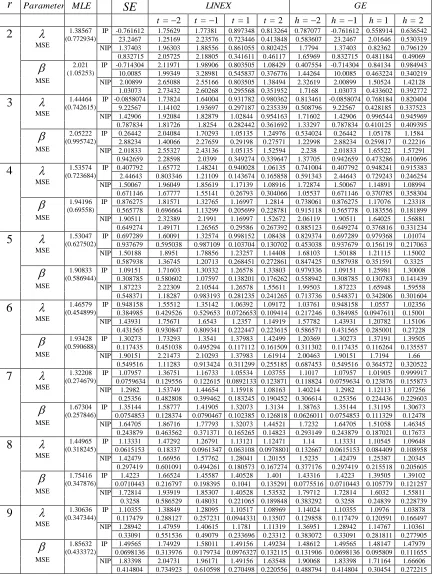
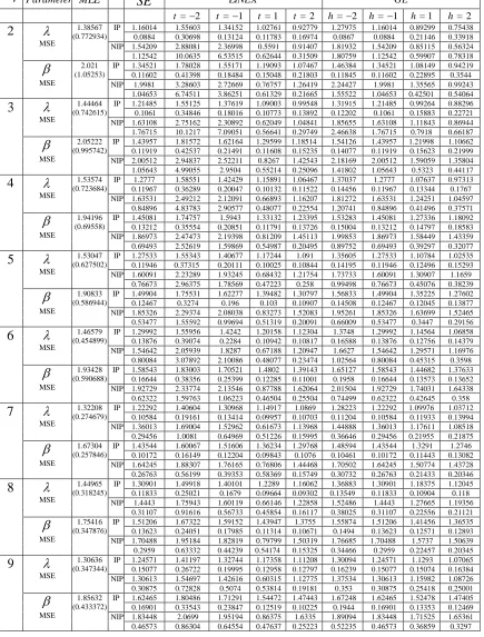
repetition 1000 times, see Tables (3.2) and (3.3).

2. Real life data example

The main idea of applying a real life data example is to determine the value of the

association parameter



. We consider the data given in Nelson (1982) for weibull

subfamily of Morgenstern family. The original data consists of

60 times to breakdown in

minutes of an insulating fluid subjected to high-voltage stress. The data is partitioned by

Nelson (1982) into six groups, each with ten insulating fluids. These data have been

analyzed by Balakrishnan et al. (2004) by assuming two-parameter exponential

distribution. We introduce here the data from groups 4 (group

X

) and 6 (group

Y

), as

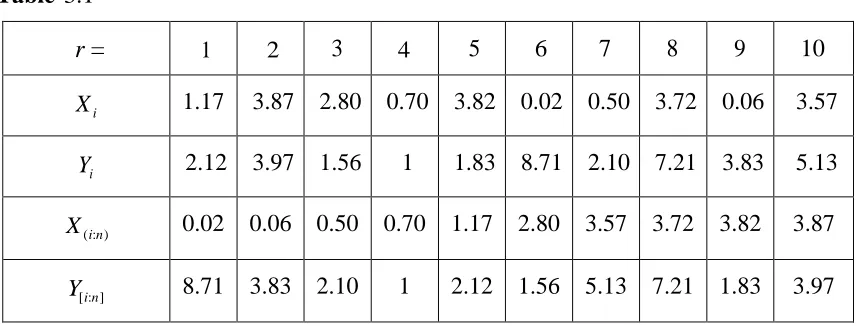
shown in Table (3.1). Based on this data, we computed the ML and Bayesian estimates of



and



under the SE, LINEX and GE loss functions using informative (with

a

₁

=

2

,

2

=

1

b

,

a

₂

=

2

,

b

₂

=

2

) and non-informative priors. We have fitted the weibull

distribution to this data, the results are as follows:



₁

=

2.5

,



₁

=

2

and



=

2.9

,



=

1.1

for group

X

and group

Y

, respectively. Since the correlation coefficient of group

X

and group

Y

is



=

0.018289

, for weibull subfamily of Morgenstern family,





=

0.2877

then



=

0.06355

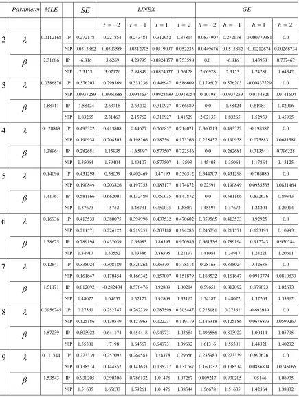
, see Tables (3.4) and (3.5).

Table

3.1

=

r

1

2

3

4

5

6

7

8

9

10

i

X

1.17 3.87 2.80 0.70 3.82 0.02 0.50 3.72 0.06 3.57

i

Y

2.12 3.97 1.56

1

1.83 8.71 2.10 7.21 3.83 5.13

) : (in

X

0.02 0.06 0.50 0.70 1.17 2.80 3.57 3.72 3.82

3.87

] : [in

Y

8.71 3.83 2.10

1

2.12 1.56 5.13 7.21 1.83

3.97

(10)

Table

3.2

r

Parameter

MLE

SE

LINEX

GE

t

=



2

t

=



1

t

=

1

t

=

2

h

=



2

h

=



1

h

=

1

h

=

2



MSE

1.38567 (0.772934)

IP -0.761612 1.75629 1.77381 0.897348 0.813264 0.787077 -0.761612 0.558914 0.636542 23.2467 1.25169 2.23576 0.723446 0.413848 0.583607 23.2467 2.01646 0.530319 NIP 1.37403 1.96303 1.88556 0.861055 0.802425 1.7794 1.37403 0.82362 0.796129 0.832715 2.05725 2.18805 0.341611 0.46117 1.65969 0.832715 0.481184 0.49069



MSE

2.021 (1.05253)

IP -0.714304 2.11971 1.98906 0.803505 1.08429 0.407554 -0.714304 0.84134 0.984943 10.0085 1.99349 3.28981 0.545837 0.376776 1.44264 10.0085 0.463224 0.340219 NIP 2.00899 2.65088 2.55166 0.803505 1.38494 2.32619 2.00899 1.50524 1.42128 1.03073 2.73432 2.60268 0.295568 0.351952 1.7168 1.03073 0.433602 0.392772

3



MSE

1.44464 (0.742615)

IP -0.0858074 1.73824 1.64004 0.931782 0.980362 0.813461 -0.0858074 0.768184 0.820404 9.22567 1.14102 1.93697 0.297187 0.235339 0.508796 9.22567 0.428185 0.337523 NIP 1.42906 1.92084 1.82879 1.02844 0.954163 1.71602 1.42906 0.996544 0.945969 0.787834 1.81726 1.8254 0.282442 0.361692 1.33297 0.787834 0.410125 0.409395



MSE

2.05222 (0.995742)

IP 0.26442 2.04084 1.70293 1.05135 1.24976 0.534024 0.26442 1.05178 1.1584 2.88234 1.40066 2.27659 0.29198 0.27571 1.22998 2.88234 0.259817 0.22216 NIP 2.01833 2.55327 2.43136 1.05135 1.52594 2.238 2.01833 1.65522 1.57291 0.942659 2.28598 2.0399 0.349274 0.339647 1.37705 0.942659 0.473286 0.410696

4



MSE

1.53574 (0.723684)

IP 0.407792 1.65772 1.48241 0.940028 1.06135 0.741004 0.407792 0.948241 0.915383 2.44643 0.803346 1.21109 0.143674 0.165858 0.591343 2.44643 0.729243 0.246254 NIP 1.50067 1.96049 1.85619 1.17139 1.08916 1.72874 1.50067 1.14891 1.08994 0.671146 1.67777 1.55141 0.26793 0.304066 1.05537 0.671146 0.370785 0.358304



MSE

1.94196 (0.69558)

IP 0.876275 1.81571 1.32765 1.16997 1.2814 0.738061 0.876275 1.17076 1.23318 0.565778 0.696664 1.13299 0.205699 0.228781 0.915118 0.565778 0.183556 0.181899 NIP 1.90511 2.32389 2.1991 1.16997 1.52672 2.06119 1.90511 1.64025 1.56881

0.649274 1.49171 1.26565 0.29586 0.267392 0.885123 0.649274 0.376816 0.331234

5



MSE

1.53047 (0.627502)

IP 0.697289 1.60091 1.32574 0.998152 1.08438 0.829374 0.697289 0.979368 1.01074 0.937679 0.595038 0.987109 0.103704 0.130702 0.453038 0.937679 0.156119 0.217063 NIP 1.50188 1.8951 1.78856 1.23257 1.14408 1.68103 1.50188 1.21115 1.15002

0.587938 1.36745 1.20713 0.268451 0.272861 0.847425 0.587938 0.351591 0.3325



MSE

1.90833 (0.586944)

IP 1.09151 1.71603 1.30332 1.26578 1.33803 0.979336 1.09151 1.25981 1.30008 0.308785 0.580602 1.07597 0.138201 0.176262 0.558942 0.308785 0.130783 0.141439 NIP 1.87223 2.22309 2.10544 1.26578 1.55611 1.99503 1.87223 1.65948 1.59558

0.548371 1.18287 0.983193 0.281235 0.241265 0.713736 0.548371 0.342806 0.301604

6



MSE

1.46579 (0.454899)

IP 0.948158 1.55512 1.35142 1.06392 1.09172 1.03761 0.948158 1.0557 1.02356 0.384985 0.429526 0.529653 0.0726653 0.109414 0.217246 0.384985 0.0947611 0.15001 NIP 1.43931 1.75671 1.6543 1.2357 1.14919 1.57782 1.43931 1.20782 1.15106 0.431565 0.930847 0.809341 0.222447 0.223615 0.586571 0.431565 0.285001 0.27228



MSE

1.93428 (0.590688)

IP 1.30273 1.73293 1.3541 1.37983 1.42499 1.20369 1.30273 1.37191 1.39505 0.117435 0.451038 0.495294 0.117112 0.161509 0.311302 0.117435 0.116264 0.135557 NIP 1.90151 2.21473 2.10293 1.37983 1.61914 2.00463 1.90151 1.7194 1.66

0.549516 1.11283 0.913424 0.311299 0.255185 0.687453 0.549516 0.364572 0.320522

7



MSE

1.32208 (0.274679)

IP 1.07957 1.36751 1.16733 1.05534 1.03755 1.1017 1.07957 1.01905 0.999917 0.0759634 0.129556 0.122615 0.0892133 0.123871 0.118824 0.0759634 0.123876 0.155873 NIP 1.2982 1.53749 1.44654 1.15918 1.08163 1.40214 1.2982 1.12113 1.07256

0.25356 0.482808 0.399462 0.183245 0.190452 0.306614 0.25356 0.224436 0.229603



MSE

1.67304 (0.257846)

IP 1.35144 1.58777 1.41905 1.32073 1.3134 1.38763 1.35144 1.31195 1.30673 0.0754853 0.128374 0.0790467 0.102385 0.126818 0.0626011 0.0754853 0.111329 0.12478 NIP 1.64705 1.86716 1.77793 1.32073 1.44521 1.7232 1.64705 1.51058 1.46345 0.243879 0.463562 0.371371 0.165265 0.14823 0.293149 0.243879 0.187021 0.17673

8



MSE

1.44965 (0.318245)

IP 1.13331 1.47292 1.26791 1.13121 1.12471 1.14 1.13331 1.10545 1.09648 0.0615153 0.18337 0.0961347 0.063108 0.0978801 0.132667 0.0615153 0.084409 0.108958 NIP 1.42479 1.66956 1.57762 1.28041 1.20155 1.5235 1.42479 1.25387 1.20345 0.297419 0.601091 0.494261 0.180573 0.167274 0.377176 0.297419 0.215518 0.205605



MSE

1.75416 (0.347876)

IP 1.4223 1.66524 1.45587 1.40528 1.401 1.43316 1.4223 1.39505 1.39102 0.0710443 0.216797 0.198395 0.1041 0.135291 0.0775516 0.0710443 0.105779 0.121257 NIP 1.72814 1.93919 1.85307 1.40528 1.53532 1.79712 1.72814 1.6032 1.55811

0.3258 0.586529 0.48031 0.221065 0.189848 0.383292 0.3258 0.24839 0.228739

9



MSE

1.30636 (0.347344)

IP 1.10355 1.38849 1.28095 1.10517 1.08969 1.14024 1.10355 1.0976 1.03878 0.117479 0.288127 0.257231 0.0944331 0.13507 0.129858 0.117479 0.120591 0.166497 NIP 1.28942 1.47959 1.40615 1.1781 1.11319 1.36951 1.28942 1.14767 1.10361

0.33091 0.551536 0.49079 0.233696 0.23312 0.383072 0.33091 0.281811 0.277905



MSE

1.85632 (0.433372)

IP 1.49565 1.74929 1.58011 1.49156 1.49234 1.48612 1.49565 1.48147 1.47979 0.0698136 0.313976 0.179734 0.0976327 0.132115 0.131906 0.0698136 0.095809 0.111655 NIP 1.83398 2.04731 1.96171 1.49156 1.63548 1.90068 1.83398 1.71164 1.66606

0.414804 0.734923 0.610598 0.270498 0.220556 0.488794 0.414804 0.30454 0.272215

(11)

Table

3.3

r

Parameter

MLE

SE

LINEX

GE

t

=



2

t

=



1

t

=

1

t

=

2

h

=



2

h

=



1

h

=

1

h

=

2



MSE

1.38567 (0.772934)

IP 1.16014 1.55603 1.34152 1.02761 0.92779 1.27975 1.16014 0.89299 0.75438 0.0884 0.30698 0.13124 0.11783 0.16974 0.0867 0.0884 0.21146 0.33918 NIP 1.54209 2.88081 2.36998 0.5591 0.91407 1.81932 1.54209 0.85115 0.56324 1.12542 10.0635 6.53515 0.62644 0.31509 1.80759 1.12542 0.59907 0.78318



MSE

2.021 (1.05253)

IP 1.34521 1.78028 1.55171 1.19093 1.07467 1.46384 1.34521 1.08149 0.94219 0.11602 0.41398 0.18484 0.15048 0.21803 0.11845 0.11602 0.22895 0.3544 NIP 1.9981 3.28603 2.72669 0.76757 1.26419 2.24427 1.9981 1.35565 0.99243 1.04653 6.74511 3.86251 0.61329 0.21665 1.55522 1.04653 0.42501 0.54064

3



MSE

1.44464 (0.742615)

IP 1.21485 1.55125 1.37619 1.09003 0.99548 1.31915 1.21485 0.99264 0.88296 0.1061 0.34846 0.18016 0.10773 0.13892 0.12202 0.1061 0.15883 0.22721 NIP 1.63108 2.75162 2.30892 0.62049 1.04841 1.85655 1.63108 1.11843 0.86944 1.76715 10.1217 7.09051 0.56641 0.29749 2.46638 1.76715 0.7918 0.66187



MSE

2.05222 (0.995742)

IP 1.43957 1.81572 1.62164 1.29599 1.18514 1.54126 1.43957 1.21998 1.10662 0.11919 0.42537 0.21491 0.11608 0.15235 0.14077 0.11919 0.15623 0.21999 NIP 2.00512 2.94837 2.52211 0.8267 1.42543 2.18169 2.00512 1.59059 1.35804 1.05643 4.99055 2.9504 0.55214 0.25096 1.41802 1.05643 0.5323 0.44117

4



MSE

1.53574 (0.723684)

IP 1.2777 1.58551 1.42429 1.15891 1.06467 1.37037 1.2777 1.07637 0.97313 0.11967 0.36289 0.20047 0.10132 0.11522 0.14456 0.11967 0.13344 0.1767 NIP 1.63531 2.49212 2.12091 0.66893 1.16207 1.81272 1.63531 1.24251 1.04597 0.84896 4.83783 2.90577 0.48077 0.22554 1.20741 0.84896 0.41496 0.37571



MSE

1.94196 (0.69558)

IP 1.45081 1.74757 1.5943 1.33132 1.23395 1.53283 1.45081 1.27336 1.18092 0.13212 0.35554 0.20851 0.11791 0.13726 0.15004 0.13212 0.14797 0.18583 NIP 1.86973 2.47473 2.19398 0.81209 1.45113 1.99853 1.86973 1.58449 1.43359 0.69493 2.52619 1.59869 0.54987 0.20495 0.89752 0.69493 0.39297 0.32077

5



MSE

1.53047 (0.627502)

IP 1.27533 1.55343 1.40677 1.17244 1.091 1.35605 1.27533 1.10784 1.02535 0.11946 0.37315 0.20111 0.10025 0.10844 0.14195 0.11946 0.12496 0.15293 NIP 1.60091 2.23289 1.93245 0.68432 1.21754 1.73733 1.60091 1.30907 1.1659 0.76673 2.96375 1.78569 0.47223 0.258 0.99498 0.76673 0.45076 0.38239



MSE

1.90833 (0.586944)

IP 1.49904 1.75531 1.62277 1.39482 1.30797 1.56833 1.49904 1.35225 1.27602 0.12467 0.3274 0.196 0.103 0.10907 0.14508 0.12467 0.12045 0.13877 NIP 1.85326 2.29374 2.08038 0.83273 1.52083 1.95261 1.85326 1.63699 1.52465 0.53477 1.55592 0.99694 0.51319 0.20091 0.66009 0.53477 0.3447 0.29156

6



MSE

1.46579 (0.454899)

IP 1.29992 1.55956 1.4242 1.20158 1.12304 1.3748 1.29992 1.14564 1.06858 0.13876 0.39074 0.2284 0.10942 0.10817 0.16588 0.13876 0.12756 0.14379 NIP 1.54642 2.05939 1.8287 0.67188 1.20947 1.6627 1.54642 1.29571 1.16976 0.80084 3.07892 2.10086 0.48077 0.23474 1.02564 0.80084 0.45315 0.3598



MSE

1.93428 (0.590688)

IP 1.58543 1.83003 1.70521 1.4802 1.39143 1.65127 1.58543 1.44682 1.37633 0.16644 0.38356 0.25399 0.12285 0.11001 0.1958 0.16644 0.13573 0.13652 NIP 1.92729 2.33774 2.13546 0.87788 1.62064 2.01504 1.92729 1.74031 1.64338 0.62322 1.59763 1.06223 0.46504 0.25504 0.74499 0.62322 0.42645 0.358

7



MSE

1.32208 (0.274679)

IP 1.22292 1.40604 1.30968 1.14917 1.0869 1.28223 1.22292 1.09976 1.03712 0.10584 0.19161 0.13414 0.09957 0.10703 0.11204 0.10584 0.11933 0.13994 NIP 1.36013 1.69004 1.52962 0.61673 1.13968 1.44888 1.36013 1.17611 1.08518 0.29456 1.0081 0.64969 0.51226 0.15995 0.36646 0.29456 0.21955 0.21875



MSE

1.67304 (0.257846)

IP 1.43544 1.60067 1.51606 1.36234 1.29768 1.48594 1.43544 1.3291 1.2746 0.10172 0.16149 0.12204 0.09843 0.1076 0.10461 0.10172 0.11443 0.13082 NIP 1.64245 1.88307 1.76165 0.76806 1.44468 1.70502 1.64245 1.50774 1.43728 0.26763 0.56199 0.39353 0.58369 0.15749 0.30732 0.26763 0.21433 0.20346

8



MSE

1.44965 (0.318245)

IP 1.30901 1.49918 1.40101 1.2289 1.16062 1.36883 1.30901 1.18375 1.12045 0.11833 0.25021 0.1679 0.09664 0.09302 0.13549 0.11833 0.10904 0.118 NIP 1.4443 1.75943 1.60119 0.66146 1.22858 1.52486 1.4443 1.27665 1.19356

0.31107 0.91616 0.56733 0.45854 0.16117 0.38025 0.31107 0.22556 0.21121



MSE

1.75416 (0.347876)

IP 1.51206 1.67322 1.59152 1.43947 1.3755 1.55874 1.51206 1.41456 1.36535 0.13623 0.24051 0.17985 0.11314 0.10671 0.1494 0.13623 0.12571 0.12893 NIP 1.70488 1.95184 1.82819 0.79799 1.50319 1.76685 1.70488 1.5737 1.50639 0.2959 0.63332 0.44239 0.54174 0.15325 0.34466 0.2959 0.22457 0.20345

9



MSE

1.30636 (0.347344)

IP 1.24571 1.41197 1.32744 1.17358 1.11208 1.30094 1.24571 1.1293 1.07065 0.15077 0.26722 0.19995 0.12958 0.12797 0.16239 0.15077 0.15074 0.16384 NIP 1.30613 1.54697 1.42616 0.60315 1.12775 1.37534 1.30613 1.15982 1.08726 0.30875 0.72828 0.5074 0.53814 0.19181 0.353 0.30875 0.25418 0.25001



MSE

1.85632 (0.433372)

IP 1.62465 1.80486 1.71291 1.54472 1.47443 1.67248 1.62465 1.52478 1.47405 0.16901 0.33543 0.23847 0.12519 0.10225 0.1944 0.16901 0.13353 0.12469 NIP 1.83448 2.0699 1.95194 0.86375 1.6335 1.89094 1.83448 1.71525 1.65361 0.46573 0.86304 0.64554 0.47637 0.25223 0.52235 0.46573 0.36859 0.3297

(12)

Table

3.4

Parameter

MLE

SE

LINEX

GE

t

=



2

t

=



1

t

=

1

t

=

2

h

=



2

h

=



1

h

=

1

h

=

2



0.0112168 IP 0.272178 0.221854 0.243484 0.312952 0.37814 0.0834907 0.272178 -0.000779381 0.0 NIP 0.0515882 0.0509568 0.0512705 0.0519097 0.052235 0.0449676 0.0515882 0.00212674 0.00268734



2.31686 IP -6.816 3.6269 4.29795 -0.0824057 0.753598 0.0 -6.816 0.43958 0.737467 NIP 2.3153 3.07176 2.94849 -0.0824057 1.56128 2.66928 2.3153 1.74281 1.64342

3



0.0386876 IP 0.376203 0.299369 0.331236 0.446947 0.586609 0.179602 0.376203 -0.00837229 0.0 NIP 0.0937259 0.0950688 0.0944634 0.0928439 0.0918054 0.10198 0.0937259 0.0144326 0.0141604



1.88711 IP -1.58424 2.63718 2.63202 0.310927 0.766589 0.0 -1.58424 0.619831 0.82016 NIP 1.83265 2.31463 2.15762 0.310927 1.41529 2.02135 1.83265 1.52939 1.45905

4



0.128849 IP 0.493322 0.413808 0.44677 0.566857 0.714071 0.360713 0.493322 -0.198587 0.0 NIP 0.190938 0.204503 0.198266 0.182561 0.173266 0.228452 0.190938 0.075883 0.0681381



1.38964 IP 0.282681 1.15935 -1.85997 0.577507 0.722546 0.0 0.282681 0.713541 0.796228 NIP 1.35064 1.59404 1.49107 0.577507 1.13593 1.45403 1.35064 1.17864 1.13125

5



0.14096 IP 0.431298 0.38059 0.402469 0.47195 0.536312 0.344707 0.431298 -0.708086 0.0 NIP 0.190849 0.203826 0.197755 0.183177 0.174872 0.22591 0.190849 0.0935535 0.0831464



1.41761 IP 0.581166 0.662001 0.132489 0.750035 0.847872 0.0 0.581166 0.832636 0.89343 NIP 1.37673 1.5752 1.48731 0.750035 1.20367 1.45597 1.37673 1.24204 1.20014

6



0.16936 IP 0.413533 0.380075 0.394998 0.437532 0.470602 0.359565 0.413533 0.92925 0.0 NIP 0.211571 0.226122 0.219255 0.203188 0.194285 0.246736 0.211571 0.123193 0.10993



1.38675 IP 0.789194 0.432039 0.66985 0.86595 0.920986 0.661356 0.789194 0.912243 0.950284 NIP 1.34917 1.50552 1.43386 0.86595 1.21197 1.41084 1.34917 1.24221 1.20611

7



0.12641 IP 0.335024 0.308189 0.320262 0.353701 0.378514 0.28165 0.335024 9.42635 0.0 NIP 0.161847 0.170454 0.166342 0.157007 0.151879 0.188532 0.161847 0.0913774 0.0810839



1.51171 IP 0.812092 -0.282434 0.578476 0.92809 1.00214 0.59651 0.812092 0.979023 1.02633 NIP 1.48072 1.64657 1.57177 0.92809 1.33162 1.54187 1.48072 1.37203 1.33362

8



0.0956745 IP 0.27361 0.252747 0.262239 0.287599 0.305447 0.223181 0.27361 -0.693989 0.0 NIP 0.125186 0.130549 0.127963 0.122231 0.119119 0.146318 0.125186 0.0676873 0.0599267



1.57239 IP 0.803922 0.641174 0.454418 0.949731 1.03684 0.496556 0.803922 1.00414 1.05795 NIP 1.55301 1.7198 1.64567 0.949731 1.39692 1.61316 1.55301 1.44321 1.40292

9



0.111544 IP 0.273339 0.257092 0.264583 0.28378 0.29656 0.235983 0.273339 0.897626 0.0 NIP 0.138514 0.144552 0.141633 0.135217 0.131767 0.160032 0.138514 0.0836804 0.0745166



1.53543 IP 0.930205 0.390306 0.786132 1.01476 1.07287 0.809217 0.930205 1.05146 1.08935 NIP 1.51635 1.65633 1.59261 1.01476 1.38544 1.56678 1.51635 1.42364 1.38832

(13)

Table

3.5

r

Parameter

MLE

SE

LINEX

GE

t

=



2

t

=



1

t

=

1

t

=

2

h

=



2

h

=



1

h

=

1

h

=

2



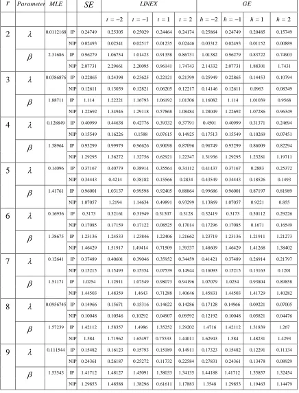
0.0112168 IP 0.24749 0.25305 0.25029 0.24464 0.24174 0.25864 0.24749 0.20485 0.15749 NIP 0.02493 0.02541 0.02517 0.01235 0.02446 0.03312 0.02493 0.01152 0.00889



2.31686 IP 0.96279 1.06754 1.01423 0.91358 0.86731 1.01382 0.96279 0.83722 0.74903 NIP 2.07731 2.29661 2.20095 0.96141 1.74743 2.14332 2.07731 1.88301 1.7431

3



0.0386876 IP 0.22865 0.24398 0.23625 0.22121 0.21399 0.25949 0.22865 0.14453 0.10794 NIP 0.12611 0.13039 0.12821 0.06205 0.12217 0.14146 0.12611 0.0963 0.08349



1.88711 IP 1.114 1.22221 1.16793 1.06192 1.01306 1.16082 1.114 1.01039 0.9568 NIP 1.22692 1.34946 1.29118 0.57868 1.08484 1.28049 1.22692 1.07286 0.96349

4



0.128849 IP 0.40999 0.44638 0.42776 0.39332 0.37791 0.4501 0.40999 0.31371 0.24694 NIP 0.15549 0.16226 0.1588 0.07615 0.14925 0.17513 0.15549 0.10269 0.07451



1.38964 IP 0.93299 0.99979 0.96626 0.90098 0.87096 0.96749 0.93299 0.86009 0.82294 NIP 1.29295 1.36272 1.32756 0.62921 1.22347 1.31936 1.29295 1.23281 1.19711

5



0.14096 IP 0.37167 0.40779 0.38914 0.35564 0.34112 0.41437 0.37167 0.2883 0.25372 NIP 0.34443 0.4214 0.38182 0.15566 0.2834 0.43549 0.34443 0.18526 0.1493



1.41761 IP 0.96001 1.03137 0.99598 0.92405 0.88864 0.99686 0.96001 0.87197 0.81989 NIP 1.07057 1.2194 1.14634 0.49891 0.93299 1.13869 1.07057 0.9221 0.855

6



0.16936 IP 0.3173 0.32161 0.31949 0.31507 0.3128 0.32419 0.3173 0.30112 0.29226 NIP 0.17085 0.17159 0.17122 0.08525 0.17014 0.17296 0.17085 0.1671 0.16549



1.38675 IP 1.23136 1.24533 1.23846 1.22406 1.21662 1.23719 1.23136 1.21911 1.21273 NIP 1.46429 1.51917 1.49414 0.71509 1.39337 1.48609 1.46429 1.41268 1.38402

7



0.12641 IP 0.37489 0.40601 0.39046 0.35952 0.34459 0.41421 0.37489 0.26914 0.21797 NIP 0.15215 0.15493 0.15354 0.07539 0.14944 0.16093 0.15215 0.13163 0.1201



1.51171 IP 1.0254 1.12911 1.07549 0.98073 0.94196 1.07079 1.0254 0.93804 0.89858 NIP 1.44503 1.48359 1.4643 0.71288 1.40646 1.45831 1.44503 1.41729 1.40282

8



0.0956745 IP 0.14966 0.15671 0.15316 0.14622 0.14286 0.17128 0.14966 0.09221 0.07005 NIP 0.10048 0.10546 0.10292 0.04907 0.09592 0.12192 0.10048 0.05821 0.04476



1.57239 IP 1.42112 1.58357 1.4986 1.35252 1.29202 1.4716 1.42112 1.31839 1.267 NIP 1.584 1.71962 1.65497 0.75533 1.44011 1.62943 1.584 1.48231 1.4293

9



0.111544 IP 0.15482 0.16123 0.15793 0.15189 0.14911 0.17323 0.15482 0.12291 0.11134 NIP 0.24361 0.26187 0.25272 0.11732 0.22584 0.27831 0.24361 0.13478 0.08929



1.53543 IP 1.41712 1.48127 1.45091 1.38033 1.34135 1.44188 1.41712 1.35857 1.32454 NIP 1.29853 1.48588 1.38296 0.61611 1.17883 1.3548 1.29853 1.19463 1.14479

(14)

4. Conclusion and comments

Based on two-parameter Weibull distribution the joint density of the concomitants of

GOS

’s for this subfamily of Morgenstern family have been discussed. The statistical

inference procedure for the unknown parameters of the given distribution such as MLE

and approximate Bayesian estimation are presented. Our applications of these results in

this model are given for concomitants of order statistics, and the estimations are

conducted on the basis of type-II censored samples. From the results in Tables (3.2) to

(3.5), we observe the following:

1.

Increasing the value of the estimated parameters does not depend on the

increasing of

r

.

2.

At

h

=



1

, we find that the Bayes estimators of the considered parameters under

GE loss functions equal to those under SE loss function.

3.

The Bayes estimators of the considered parameters under LINEX and GE loss

functions give more accurate results than MLE estimator and those under SE loss

function by increasing and decreasing the values of

t

and

h

respectively.

4.

For considering various values for the hyperparameters in the informative priors

of Bayes estimators, the results did not change the obtained conclusions.

5.

The Bayes estimators of the considered parameters obtained from MCMC method

give more accurate results than Lindley’s approximation, with considering that

Lindley’s approximation give in some results negative and complex values.

6.

In the simulation study, the results obtained from IP are more accurate than NIP

for the Bayes estimators of



and



.

7.

In the real life data study, the results obtained from NIP are more accurate than IP

for the Bayes estimators of



and



.

The proposed procedures for the estimation problems may be considered for other models

and distributions.

Conflict of interest

The authors declare that they have no conflict of interest.

Acknowledgments

The authors would like to thank the anonymous referees for their constructive comments

on an early version of this paper.

References

1.

Balakrishnan, N., Lin, C.T. and Chan, P.S. (2004). Exact inference and prediction

for k-sample two-parameter exponential case under general Type-II censoring.

Journal of Statistical Computation and Simulation

, 74,

867



878

.

(15)

3.

David, H.A., O’Connell, M.J. and Yang, S.S. (1977). Distribution and expected

value of the rank of a concomitant of an order statistic.

Annals of Statistics

, 5,

223

216



.

4.

Dey, D.K., Ghosh, M. and Srinivasan, C. (1987). Simultaneous estimation of

parameters under entropy loss.

Journal of Statistical Planning and Inference

, 25,

363

347



.

5.

Dey, D.K. and Liu, P.L. (1992). On comparison of estimators in a generalized life

model.

Microelectronics Reliability

, 33,

207



221

.

6.

Jaheen, Z.F. (2004a). Empirical Bayes inference for generalized exponential

distribution based on records.

Communications in Statistics-Theory and Methods

,

33 (8),

851

1861

.

7.

Jaheen, Z.F. (2004b). Empirical Bayes analysis of record statistics based on linex

and quadratic loss functions.

Computers and Mathematics with Applications

, 47,

954

947



.

8.

Johnson, N.L. and Kotz, S. (1975). On some generalized

Farlie-Gumbel-Morgenstern distributions.

Communications in Statistics-Theory and Methods

, 4,

427

415



.

9.

Kamps, U. (1995). A concept of generalized order statistics.

Journal of Statistical

Planning and Inference

, 48,

1

23

.

10.

Lindley, D.V. (1980). “Approximate Bayes methods”.

Trabajos de Estatadistica

,

31,

223

237

.

11.

Metropolis, N., Rosenbluth, A.W., Rosenbluth, M.N., Teller, A.H. and Teller, E.

(1953).“Equation of state calculations by fast computing machines”.

The Journal

of Chemical Physics

, 21 (6),

1087



1092

.

12.

Mohie EL-Din, M.M., Amein, M.M., Ali, N.S.A. and Mohamed, M.S. (2015). On

joint density for concomitants of generalized order statistics based on

Morgenstern family. Submitted.

13.

Nelson, W. (1982).

Applied Life Data Analysis

. John Wiley & Sons, New York,

462.

14.

Singh, U., Gupta, P.K. and Upadhyay, S. (2002). Estimation of exponentiated

Weibull shape parameter under linex loss function.

Communications in

Statistics-Simulation and Computation

, 31,

523



537

.

15.

Soliman, A.A. (2005). Estimation of parameters of life from progressively

censored data using Burr-XII Model.

IEEE Transactions on Reliability

, 54 (1),

42

34



.

16.

Soliman, A.A. (2006). Estimators for the finite mixture of Rayleigh model based

on progressively censored data.

Communications in Statistics-Theory and

Methods

, 35 (5),

803



820

.