SEARCH STRATEGY FOR NESTED LOGIT TREE STRUCTURE:
A CASE STUDY OF RURAL FEEDER SERVICE TO BUS STOP
Sudhanshu Sekhar Das1, Santanu Ghosh2, Bhargab Maitra3, Manfred Boltze4
1 RSR Rungta College of Engineering and Technology, Bhilai, India
2, 3 Department of Civil Engineering, Indian Institute of Technology Kharagpur, Kharagpur – 721302, India 4 Transport Planning and Traffic Engineering, Darmstadt University of Technology, Petersenstr. 30, 64287 Darmstadt, Germany
Received 25 June 2012; accepted 19 September 2012
Abstract: Several approaches have been suggested by researchers for identifying the best
feasible tree structure for Nested Logit (NL) model. This paper demonstrates an experience of applying those approaches while identifying the best feasible tree structure for NL model with reference to a case study of feeder service to bus stop in rural India. Heteroscedastic Extreme Value (HEV) model, fully degenerated tree structure NL (DGNL) model and several nested logit models based on natural partition principle were developed and analyzed for identifying the most optimal NL model. The results presented in the paper are case specific but the experiences documented could be useful for selecting the optimal tree structure for NL model in other cases.
Keywords: choice model, travel behaviour analysis, Nested Logit, tree structure, Heteroscedastic Extreme Value model.
3 Corresponding author: [email protected]
1. Introduction
Choice models are used in transportation and other fields to represent the selection of one among a set of mutually exclusive alternatives. Multinomial logit (MNL) model (McFadden, 1974) is the most widely used choice model due to its simple mathematical structure and ease in estimation. However, MNL imposes restriction, that the distribution of random error term is independent and identically distributed over alternatives (IID). This restriction leads to independence of irrelevant alternative (IIA) property which causes the cross elasticity across all pairs of alternative to be same and therefore, may result into biased outcomes. Most widely known closed formed model,
which relaxes restrictions of MNL model, is the nested logit (NL) model (Williams, 1977). Over the last few decades several works have been reported in the literature on theoretical improvement and application NL models for the empirical analysis of travel behavior (Manheim, 1973; Williams, 1977; McFadden, 1978; Hensher, 1998; Bliemer et al., 2009; Das et al., 2009; Dissanayake and Morikawa, 2010; Lee and Waddell, 2010; Siriwardena et al., 2012).
tree structure upon which to condition the analysis in an econometric sense with best feasible solution. This paper demonstrates an experience of identifying the best feasible tree structure for NL model with reference to a case study of feeder service to bus stop in rural India.
Das et al. (2009) investigated the valuation of attributes of rural feeder service with reference to a case study of about 200 square-km area in the state of West Bengal, India. The study area is bounded by National Highway (NH) in the Eastern side, Major District Roads (MDRs) in Northern and Western sides, and river Subarnarekha in the Southern side. Presently, the study area is served by twelve bus stops, which are located on the NH and MDRs. However, the roads within the study area are not served by any feeder system so far. The database developed by Das et al. (2009) is used in the present work for demonstrating the experience of identifying the best feasible tree structure for NL model. It may be mentioned that Das et al. (2009) also included a NL model while comparing the valuation of travel attributes using different econometric model specifications. However, the work did not address in specific the issues pertaining to identifying the best feasible tree structure for NL model, which is the focus of the present work.
2. Methodology
The methodology includes collection of behavioral data from commuters, and development of utility equations using Nested logit model specifications. The details of feeder service, design of survey instrument, collection of data and development of database have been reported by Das et al. (2009). However, a brief outline of the same in the context of the present paper is given below.
2.1. Feeder Services
Feeder services are described with reference to ‘type of vehicle’ and ‘form of operation’. Two feeder vehicles namely ‘Tempo’ with capacity of 6 persons (called as Vehicle-I) and ‘Trekker’ with capacity of 10 persons (called as Vehicle-II) are considered. The travel demand in rural areas is normally distributed over a large geographical area. Therefore, along with ‘Fixed-Schedule’, two flexible forms of operation namely Ride’ and ‘Dial-a-Slot’, are also investigated in the context of rural feeder service to bus stop.
In ‘Fixed-Schedule’, the arrival/departure of next vehicle is known to commuters but the availability of seat is not assured (due to limited vehicle capacity). As the seat availability or travel opportunity in the very next vehicle is not assured, the waiting time is described as ‘anxious waiting at stop’. In ‘Dial-a-Ride’, a passenger is assumed to inform service provider about the origin and the destination for a ride along the route using toll free telephone available at stop. In response, service provider informs the passenger about the vehicle allotted for the trip, but starts the vehicle only when capacity utilization of the vehicle along the route is assured to a desired level. Therefore, both operator and commuters are benefited. The operator provides the service with desired utilization of seat capacity and commuters are benefited as the seat availability is assured in specified vehicle. As the seat availability is assured in a specified vehicle, the waiting is described as ‘Relaxed Waiting at Stop’.
number from home end. The service provider collects all such requests, schedules a vehicle ensuring acceptable usage of vehicle capacity along the route, and informs users about the allocated time slot and vehicle. In the process, some commuters may be allocated time slots other than the requested ones. Deviation from requested time slot, if any, is considered as disutility to commuters. As seat availability is assured in specified vehicle and arrival time is also known, commuters can wait at home end. Accordingly, the time deviation or waiting is considered as ‘Relaxed Waiting at Home End’.
2.2. Database
The attributes considered for design of stated choice (SC) experiment included fare, access walking distance, seating discomfort (within a vehicle), time deviation (i.e. time difference between intended and actual start of journey), and waiting discomfort. It may be mentioned that traveling as standee is not a viable option for feeder vehicles considered in the present work. However, often in rural India such vehicles are found to carry more passengers than the seat capacity specified by vehicle manufacturer(s). Traveling under
such a condition causes additional discomfort to passengers and accordingly the travel was described as ‘congested seating’. When vehicles carry passenger only upto the seat capacity specified by manufacturer, the travel was described as ‘comfortable seating’. Attributes and their levels considered for SC experimentation are given in Table 1.
A full factorial design (Louviere et al., 2000) with all the attributes and their levels mentioned in Table 1 would have produced 384 alternatives. However, it was neither necessary nor practically possible to include all these combinations in the SC experiment. Therefore, some alternatives were eliminated using fractional factorial technique (Green et al., 2001). Fractional factorial orthogonal design using SPSS 7.5 (as described in Hensher et al., 2005) was used to produce 16 alternatives. These alternatives were used to prepare 10 choice sets, each containing 6 SC alternatives in an alternative specific form to represent three forms of operation (i.e. fixed-schedule, dial-a-ride and dial-a-slot) each with two alternative vehicles (i.e. Vehicle-I and Vehicle-II).
Stratified random sampling technique (Hensher, 1994) based on occupation of
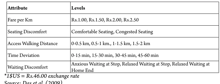
Table 1
Attributes and their Levels
Attribute Levels
Fare per Km Rs.1.00, Rs.1.50, Rs.2.00, Rs.2.50
Seating Discomfort Comfortable Seating, Congested Seating
Access Walking Distance 0-0.5 km, 0.5-1 km., 1-1.5 km, 1.5-2 km
Time Deviation 0-15 min, 15-30 min, 30-45 min, 45-60 min
Waiting Discomfort Anxious Waiting at Stop, Relaxed Waiting at Stop, Relaxed Waiting at Home End
head of the household was used for the selection of sample for household-survey in the SC experiment. The responses were collected from the heads of the households. During pilot surveys, 3 choice sets containing 6 alternatives were included in questionnaire. However, majority of respondents reported difficulties in selecting one among 6 alternatives presented to them. Considering the fact that rural respondents were exposed to such type of survey for the first time, it was decided to conduct choice experiment in a sequential manner with four steps (Das et al., 2009).
• Step-1: Choose one from four alternatives representing fixed-schedule and dial-a-ride each with two alternative vehicles
• Step-2: Choose one from four alternatives representing fixed-schedule and dial-a-slot each with two alternative vehicles
• Step-3: Choose one from four alternatives representing dial-a-ride and dial-a-slot each with two alternative vehicles
• Step-4: Choose one from six alternatives representing fixed-schedule, a-ride, dial-a-slot each with two alternative vehicles
Respondents, who were initially unable to choose one from six alternatives, were comfortable to give their choices when sequential approach was followed. Choices indicated by a respondent in sequential approach were also helpful for checking the consistency of choices made by the respondent. However, in order to avoid fatigue (Carson et al., 1994), only one choice set containing six alternatives with its sequences was included in the questionnaire. Although 998 responses were obtained during data collection, some of the responses were omitted during the refinement of database and finally 674 responses i.e. 674 choice sets were included in the final database.
2.3. Econometric Models
The stated choice data is analyzed by developing econometric models (McFadden, 1978; Ben-Akiva and Lerman, 1985; Borsch-Supan, 1990). The theoretical backgrounds of these models are available in the literature. However, a brief outline of models used in the present work is given below.
In econometric models based on Random Utility Theory (McFadden, 1974), the utility of each element (k) consists of an observed (deterministic) component denoted by V and a random (disturbance) component denoted by ε (Eq. (1)):
Uk = Vk + εk (1)
The deterministic part Vk is again a function
of the observed attributes (x) of the choice as faced by the individual (t), the observed socioeconomic attributes of the individual (s) and a vector of parameters (β), then (Eq. (2)):
Vk = Vk (x, s, β) (2)
A probabilistic statement can be made (due to presence of the random component) as, when an individual ‘t’ is facing a choice set, Ck, consisting of Jk choices, the choice
probability of alternative i is equal to the probability that the utility of alternative ‘i’, Uik, is greater than or equal to the utilities
of all other alternatives in the choice set. i.e.
Pk (i) = Pr (Uik ≥ Ujk, for all j Cn)
Pk (i) = Pr (Vik + εik ≥ Vjk + εjk, for all j Ck, j ≠i)
1985) (Eq. (3)):
(3)
This model can be estimated by Maximum Likelihood techniques, and is useful for modeling choice behavior.
The NL model arises as a random utility model in which the random component of utility has the generalized extreme value distribution which relaxes IIA partially. In NL each observed (or representative) component of the utility expression for an alternative (Vk for kth alternative)
is defined in the terms of four parts – the vector parameters (β) associated with explanatory variable, an alternative specific constant (αk), a scale parameter (θ), and the explanatory
variable (x). The utility of alternative ‘k’ for individual ‘t’ is (Eq. (4)):
(4)
Var[εtk] = σ 2 = κ/θ2
The scale parameter (θ), is proportional to inverse of the standard deviation (σ) of the random component in the utility expression, and is critical input into the set up of the NL model (Ben-Akiva and Lerman, 1985; Louviere et al., 2000). In order to be consistent with utility maximization, the scale parameters at highest level and the ratios of scale parameters at each lower nest are bounded by zero and one. The same observed set of choices emerges regardless of the (common) scaling of the utilities. Hence, the latent variance is normalized to one, not as a restriction, but as the necessity for identification (Hensher and Greene, 2002). To be consistent with McFadden random utility maximization nested logit model normalization is also required (Koppelman and Wen, 1998; Hensher and Greene, 2002). Normalization is simply the process of setting one or more scale parameters equal to unity, while allowing the other scale parameters to be estimated. Estimation of NL models uses full information maximum likelihood to increase estimation efficiency and allows imposing constraints on utility function parameters in different nest structures (Brownstone and Small, 1989; Hensher, 1991). Defining parameter vectors in the utility functions at each level as ‘b’ for elemental alternatives, ‘g’ for branch composite alternatives, and ‘d’ for limb composite alternatives and normalizing the scale parameter in the elemental (lowest level) level in a three level tree structure (Fig. 1 and Fig. 2), the conditional choice probabilities for the elemental alternatives (k) is defined as Eq. (5):
where k|ji = elemental alternative k in branch j of limb i, K|ji = number of elemental alternatives in branch j of limb i, and the inclusive value for branch j in limb i is (Eq. (6)):
(6)
The branch level probability is (Eq. (7)):
(7)
where j|i = branch j in limb i, J|i = number of branches in limb i, and (Eq. (8)):
(8)
Finally, the limb level is defined by Eq. (9):
(9)
where I = number of limbs in the three level tree and (Eq. (10)):
(10)
The unconditional probability of an elemental alternative, by law of probability (Eq. (11)): (11)
HEV can be used as a search engine for NL tree structure in an econometric sense (Hensher, 1998). Without going through theoretical detail, the choice probability of the individual choosing an element ‘k’ in HEV model (Bhat, 1995) can be expressed as Eq. (12):
(12)
Where, θiand θj are scale parameter for the ith and jth alternative, w=εi / θi. The integral does
3. Model Development
The attributes which were taken for development of logit models using NLOGIT 4.0 (2007) included,
• Type (Effect coded: 1 for Vehicle-II and -1 for Vehicle-I)
• System1 (Effect coded: 1 for ‘dial-a-slot’, 0 ‘for dial-a-ride’ and -1 for ‘fixed schedule’)
• System2 (Effect coded: 0 for ‘dial-a-slot’, 1 ‘for dial-a-ride’ and -1 for ‘fixed schedule’)
• Seating Discomfort (Effect coded: -1 for Congested Seating, and 1 for Comfortable Seating)
• Walking distance in meter (Cardinal linear)
• Anxious waiting time at bus stop in minute (Cardinal linear)
• Relax waiting time at bus stop in minute (Cardinal linear)
• Relaxed waiting time at home end in minute (Cardinal linear)
• Fare per kilometer in Paise (100 Paise = 1 INR) (Cardinal linear).
Initially, a MNL model (called as MNL1 in
Table 2) was estimated with all the parameters. However, as t-vales of all parameter estimates except for ‘System1’ and ‘System2’ were found
significant, the model was re-estimated (called as MNL2 in Table 2) ignoring ‘System1’ and
‘System2’. All the parameters estimates of MNL2
were found statistically significant with logical signs of the estimates. The negative signs of the quantitative attributes indicate that the utility of trip makers decreases with an increase in the magnitude of respective attributes. For the qualitative attribute ‘Seating Discomfort’, positive sign indicates that changing from ‘comfortable seating’ to ‘congested seating’ decreases the utility. Similarly, negative sign associated with the estimate of ‘Type’ indicates trip makers’ preferences towards Vehicle-II over Vehicle-I. The overall goodness of fit was
considered using ρ2. Value of the ρ2 between
0.2 and 0.4 indicates acceptable model fit (Louviere et al., 2000). Therefore, MNL2
model was accepted for further analysis.
All parameters of MNL2 were taken for the
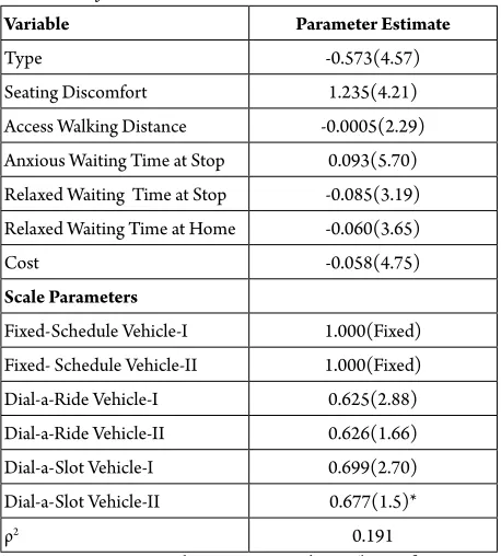
development of the Nested Logit (NL) model. Regarding the decision of tree structure upon which to condition the analysis, Hensher (1998) proposed the use of Heteroscedastic Extreme Value (HEV) model for identifying the most likely NL model tree structure. Several trials were made to get the convergence of HEV model with desirable signs for all the parameter estimates. The convergence of the HEV model was obtained when the scale parameters of fixed schedule alternatives (i.e. Fixed-schedule Vehicle-I and Fixed-schedule Vehicle-II) were restricted to unity (Table 3). All the t-statistics of parameter estimates except the scale parameter of Dial-a-Slot Vehicle-II from HEV model were found statistically significantly different from zero at 95% confidence level. The results indicated the possibility of a system based tree structure containing fixed schedule form of operation in one leg and flexible form of operation in the other leg (Fig. 1; Table 5) due to similar value of scale parameter. However, due to the restriction imposed on the scale parameter, no definite conclusion could be made from the results.
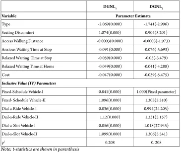
HEV models are generally well known for their failure in convergence (Hensher et al., 2005). Acknowledging this fact Hensher et al. (2005) suggested the use of a fully degenerated tree structure NL model and resulting inclusive value (IV) parameters as guidance for deciding the final tree structure to be adopted for NL. Fully degenerated NL (DGNL) model, one without constraining any IV parameter (called as DGNL1
in Table 4) and the other with constraining IV parameter of fixed Schedule Vehicle-I to ‘1’ (called as DGNL2 in Table 4) were developed
Table 2
Estimation of MNL Model Results
Variable MNL1 MNL2
System1 -0.124 (-0.56)
System2 0.157 (0.53)
Type -0.608 (-8.92) -0.601 (-9.26)
Seating Discomfort 1.08 (9.32) 1.083 (9.45)
Access Walking Distance -0.00037 (-2.67) -0.00039 (-2.87)
Anxious Waiting Time at Stop -0.093 (-9.64) -0.093 (-11.09)
Relaxed Waiting Time at Stop -0.07 (-5.64) -0.065 (-9.10)
Relaxed Waiting Time at Home -0.051 (-5.45) -0.054 (-8.50)
Cost -0.049 (-13.8) -0.049 (-14.02)
Log likelihood function -747.638 -747.829
ρ2 0.204 0.204
Note: t-statistics are shown in parenthesis Source: Das et al. (2009)
Table 3
Estimation of HEV Model Results
Variable Parameter Estimate
Type -0.573(4.57)
Seating Discomfort 1.235(4.21)
Access Walking Distance -0.0005(2.29)
Anxious Waiting Time at Stop 0.093(5.70)
Relaxed Waiting Time at Stop -0.085(3.19)
Relaxed Waiting Time at Home -0.060(3.65)
Cost -0.058(4.75)
Scale Parameters
Fixed-Schedule Vehicle-I 1.000(Fixed)
Fixed- Schedule Vehicle-II 1.000(Fixed)
Dial-a-Ride Vehicle-I 0.625(2.88)
Dial-a-Ride Vehicle-II 0.626(1.66)
Dial-a-Slot Vehicle-I 0.699(2.70)
Dial-a-Slot Vehicle-II 0.677(1.5)*
ρ2 0.191
Table 4
Estimation of DGNL Model Results
DGNL1 DGNL2
Variable Parameter Estimate
Type -2.069(0.000) -1.741(-2.996)
Seating Discomfort 1.074(0.000) 0.904(5.201)
Access Walking Distance -0.0003(0.000) -0.0003(-1.973)
Anxious Waiting Time at Stop -0.091(0.000) -0.076(-5.693)
Relaxed Waiting Time at Stop -0.059(0.000) -0.05(-3.479)
Relaxed Waiting Time at Home -0.049(0.000) -0.041(-4.288)
Cost -0.047(0.000) -0.039(-5.475)
Inclusive Value (IV) Parameters
Fixed-Schedule Vehicle-I 0.841(0.000) 1.000(Fixed parameter)
Fixed- Schedule Vehicle-II 1.096(0.000) 1.303(5.510)
Dial-a-Ride Vehicle-I 0.836(0.000) 0.994(24.205)
Dial-a-Ride Vehicle-II 1.12(0.000) 1.331(5.157)
Dial-a-Slot Vehicle-I 0.856(0.000) 1.018(27.945)
Dial-a-Slot Vehicle-II 1.099(0.000) 1.306(5.541)
ρ2 0.208 0. 208
Note: t-statistics are shown in parenthesis
Vehicle-I
Demand Responsive Fixed Scheduled
Dial-a-Slot Dial-a-Ride
Travel
Vehicle-II
Vehicle-II Vehicle-II
Vehicle-I Vehicle-I
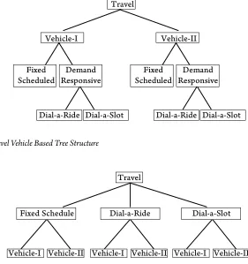
Fig. 2.
Three Level Vehicle Based Tree Structure
Fig. 3.
Two Level System Based Tree Structure
Fig. 4.
Two Level Vehicle Based Tree Structure
Fixed
Scheduled ResponsiveDemand
Travel
Dial-a-Ride Dial-a-Slot
Vehicle-I Vehicle-II
Fixed
Scheduled ResponsiveDemand
Dial-a-Ride Dial-a-Slot
Fixed Schedule
Vehicle-I
Dial-a-Slot Dial-a-Ride
Vehicle-II
Travel
Vehicle-I Vehicle-II Vehicle-I Vehicle-II
Fixed
ScheduledDial-a-Ride Dial-a-Slot Travel
Vehicle-I
Fixed
The estimated value of IV parameters in DGNL model indicated that ‘Vehicle-I’ and ‘Vehicle-II’ of all forms of operation were almost of similar value. It showed an existence of relationship between Vehicle-I and Vehicle-II of all operating systems. So, a vehicle based tree structure was identified as a viable tree structure option with two possibilities (Fig. 2 and Fig. 4). Greene (2000) argued that there would often be a natural partition of the alternatives that can guide estimation. However, when there
are many alternatives faced by consumers, several tree structures might be possible based on natural partition principle. In the present case, all four possible tree structures guided by natural partition were attempted as per Figs. 1-4 in order to verify the claim of the DGNL model. The corresponding NL models are called as NL1, NL2, NL3 and NL4
in Table 5. All the parameters of MNL2 were
included in the utility of the lower level with normalizing scale parameter in the elemental level (lower level).
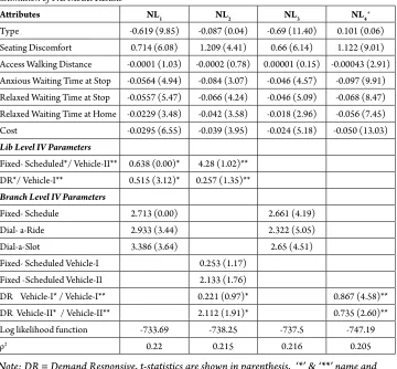
Table 5
Estimation of NL Model Results
Attributes NL1 NL2 NL3 NL4+
Type -0.619 (9.85) -0.087 (0.04) -0.69 (11.40) 0.101 (0.06)
Seating Discomfort 0.714 (6.08) 1.209 (4.41) 0.66 (6.14) 1.122 (9.01)
Access Walking Distance -0.0001 (1.03) -0.0002 (0.78) 0.00001 (0.15) -0.00043 (2.91)
Anxious Waiting Time at Stop -0.0564 (4.94) -0.084 (3.07) -0.046 (4.57) -0.097 (9.91)
Relaxed Waiting Time at Stop -0.0557 (5.47) -0.066 (4.24) -0.046 (5.09) -0.068 (8.47)
Relaxed Waiting Time at Home -0.0229 (3.48) -0.042 (3.58) -0.018 (2.96) -0.056 (7.45)
Cost -0.0295 (6.55) -0.039 (3.95) -0.024 (5.18) -0.050 (13.03)
Lib Level IV Parameters
Fixed- Scheduled*/ Vehicle-II** 0.638 (0.00)* 4.28 (1.02)**
DR*/ Vehicle-I** 0.515 (3.12)* 0.257 (1.35)**
Branch Level IV Parameters
Fixed- Schedule 2.713 (0.00) 2.661 (4.19)
Dial- a-Ride 2.933 (3.44) 2.322 (5.05)
Dial-a-Slot 3.386 (3.64) 2.65 (4.51)
Fixed- Scheduled Vehicle-I 0.253 (1.17)
Fixed -Scheduled Vehicle-II 2.133 (1.76)
DR Vehicle-I* / Vehicle-I** 0.221 (0.97)* 0.867 (4.58)**
DR Vehicle-II* / Vehicle-II** 2.112 (1.91)* 0.735 (2.60)**
Log likelihood function -733.69 -738.25 -737.5 -747.19
ρ2 0.22 0.215 0.216 0.205
In NL1 model, access walking distance, some
lib level IV parameters and branch level IV parameters were insignificant. Similarly, in NL2
model access walking distance, all lib level IV parameters and branch level IV parameters were insignificant. Access walking distance in NL3 was
insignificant. After comparison of all the NL models, the NL4 model with a two level vehicle
base tree structure (Fig. 4) was accepted as all important attributes describing the feeder service and IV parameters were significant and with proper sign. This findings supports the claim of DGNL model i.e. existence of vehicle based tree structure. In the present case, DGNL model was found useful to narrow down the search domain to only a few possible tree structures (Fig. 2 and Fig. 4) rather that investigating all possible tree structures guided by natural partition only. In vehicle base tree structure, differences between the vehicles are captured through IV parameters, hence the vehicle specific variable in NL4 was
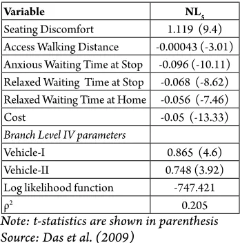
found insignificant. So another NL model called as NL5 (Table 6) was developed neglecting vehicle
specific variable ‘Type’. The NL5 model is accepted
considering significance and signs of parameter estimates. Estimates of NL5 are also in conformity
with MNL2 and random utility maximization.
Table 6
Estimation of Accepted NL Model Results
Variable NL5
Seating Discomfort 1.119 (9.4)
Access Walking Distance -0.00043 (-3.01)
Anxious Waiting Time at Stop -0.096 (-10.11) Relaxed Waiting Time at Stop -0.068 (-8.62) Relaxed Waiting Time at Home -0.056 (-7.46)
Cost -0.05 (-13.33)
Branch Level IV parameters
Vehicle-I 0.865 (4.6)
Vehicle-II 0.748 (3.92)
Log likelihood function -747.421
ρ2 0.205
Note: t-statistics are shown in parenthesis Source: Das et al. (2009)
4. Conclusion
An important issue related to Nested Logit (NL) modeling is the decision of tree structure upon which to condition the analysis so as to get the best feasible solution. Several approaches have been suggested by researchers for identifying the best feasible tree structure for NL model. This paper demonstrates an experience of applying those approaches while identifying the best feasible tree structure for NL model with reference to a case study of feeder service to bus stop in rural India. The case study includes various attributes of rural feeder service with two types of feeder vehicle and three forms of operation.
HEV models are generally considered to be notorious because of failure in convergence. In the present case study, the behavioral data could be analyzed by developing a HEV model. The results indicated the possibility of a system based tree structure containing fixed schedule form of operation in one leg and flexible form of operation in the other leg due to similar value of scale parameters. However, due to the restriction imposed on the scale parameter, no definite conclusion could be made from the results.
i.e. DGNL model and natural partition principle can be used together in sequence for identifying the best feasible tree structure with optimal modeling efforts. While DGNL model may be instrumental in narrowing down the search domain, the natural partition principle can be useful in identifying the specific optimal tree structure within the search domain. The results presented in the paper are case specific but the experiences documented could be useful for selecting the optimal tree structure for NL model in other cases.
Acknowledgment
The work presented in this paper is carried out with support from Deutscher Akademischer Austausch Dienst (DAAD) and Alexander von Humboldt Stiftung. Authors express their sincere thanks to these institutions for their support towards international exchange and research.
References
Ben-Akiva, M.; Lerman, S.R. 1985. Discrete Choice Analysis: Theory and Applications to Travel Demand. MIT Press, Cambridge.
Bhat, C.R. 1995. A heteroscedastic extreme value model of intercity travel mode choice, Transportation Research Part B. DOI: http://dx.doi.org/10.1016/0191-2615(95)00015-6, 29(6): 471-483.
Bliemer, M.C.J.; Rose, J.M.; Hensher, D.A. 2009. Efficient stated choice experiments for estimating nested logit models, Transportation Research Part B. DOI: http://dx.doi. org/10.1016/j.trb.2008.05.008,43(1): 19-35.
Borsch-Supan, A. 1990. On the Compatibility of Nested Logit Models with Utility Maximization, Journal of
Econometrics. DOI:
http://dx.doi.org/10.1016/0304-4076(90)90126-E, 43(3): 373-388.
Brownstone, D.; Small, K.A. 1989. Efficient Estimation of Nested Logit Model, Journal of Business and Economic
Statistics. DOI: http://dx.doi.org/10.1080/07350015.1
989.10509714, 7(1): 67-74.
Carson, R.; Louviere, J.J.; Anderson, D.A.; Arabie, P.; Bunch, D.S.; Hensher, D.A.; Johnson, R.M.; Kuhfeld, W.F.; Steinberg, D.; Swait, J.; Timmemans, H.; Wiley, J.B. 1994. Experimental analysis of choice, Marketing
Letters. DOI: http://dx.doi.org/10.1007/BF00999210,
5(4): 351-368.
Das, S.S.; Maitra, B.; Boltze, M. 2009. Valuing Travel Attributes of Rural Feeder Service to Bus Stop: A Comparison of Different Logit Model Specifications, Journal of Transportation Engineering, ASCE. DOI: http://dx.doi. org/10.1061/(ASCE)0733-947X(2009)135:6(330), 135(6): 330-337.
Dissanayake, D.; Morikawa, T. 2010. Investigating household vehicle ownership, mode choice and trip sharing decisions using a combined revealed preference/stated preference Nested Logit model: case study in Bangkok Metropolitan Region. Journal of Transport Geography. DOI: http://dx.doi.org/10.1016/j.jtrangeo.2009.07.003, 18(3): 402-410.
Green, P.E.; Krieger, A.M.; Wind, Y.J. 2001. Thirty Years of Conjoint Analysis: Reflections and Prospects, Interfaces. DOI: http://dx.doi.org/10.1287/inte.31.3s.56.9676, 31(3): 56-73.
Greene, W. 2000. Econometric Analysis. 4th ed. Prentice Hall, Upper Saddle River.
Hensher, D.A. 1991. Efficient Estimation of Hierarchical Logit Mode Choice Model. In Proceedings of theJapanese Society of civil Engineering. 17-28.
Hensher, D.A. 1994. Stated Preference Analysis of Travel Choices: The State of Practice, Transportation. DOI: http:// dx.doi.org/10.1007/BF01098788, 21(2): 107-133.
Hensher, D.A. 1998. HEV Choice Models as a Search Engine for Specification of Nested Logit Tree Structure, Marketing Letter. DOI: http://dx.doi. org/10.1023/A:1008151702729, 10(4): 333-343.
Hensher, D.A.; Rose, J.M.; Greene, W.H. 2005. Applied Choice Analysis a Primer. Cambridge University Press.
Koppelman, F.S.; Wen, C. 1998. Alternative Nested Logit Models: Structure, Properties and Estimation,
Transportation Research Part B. DOI: http://dx.doi.
org/10.1016/S0191-2615(98)00003-4, 32(5): 289-298.
Lee, B.H.Y.; Waddell, P. 2010. Residential mobility and location choice: a nested logit model with sampling of alternatives, Transportation. DOI: http://dx.doi. org/10.1007/s11116-010-9270-4, 37(4): 587-601.
Louviere, J.J.; Hensher, D.A.; Swait, D.J. 2000. Stated Choice Methods. Analysis and Applications. Cambridge University Press.
Manheim, M.L. 1973. Practical Implications of Some Fundamental Properties of Travel Demand Models,
Highway Research Record, 422: 21-38.
McFadden, D. 1974. Conditional Logit Analysis of Qualitative Choice Behavior, In P. Zarembka (ed.), Frontiers in econometrics, New York: Academic Press. 105-142.
McFadden, D. 1978. Modelling the Choice of Residential Location, Transportation Research Record. 672: 72-77.
NLOGIT 4.0. 2007. Reference Guide. Econometrics Software Inc.
Siriwardena, S.; Hunt, G.; Teisl, M.F.; Noblet, C.L. 2012. Effective environmental marketing of green cars: A nested-logit approach, Transportation Research Part D. DOI: http:// dx.doi.org/10.1016/j.trd.2011.11.004, 17(3): 237-242.
Williams, H.C.W.L.; Senior, M.L. 1977. Model Based Transport Policy Assessment II: Removing Fundamental Inconsistencies from the Models, Traffic Engineering and Control, 18(10): 464-469.
STRATEGIJA PRETRAGE STRUKTURE
STABLA OBUHVATNOG LOGIT MODELA:
STUDIJA SLUČAJA SABIRNOG PREVOZA
PUTNIKA DO AUTOBUSKOG STAJALIŠTA
U RURALNIM PODRUČJIMA
Sudhanshu Sekhar Das, Santanu Ghosh, Bhargab Maitra, Manfred Boltze
Sažetak: Autori prikazanog istraživanja prepor učuju nekoli ko pr i stupa za identifikaciju najpodesnije strukture stabla obuhvatnog logit modela. Ovaj rad ilustruje iskustvo primene ovih pristupa prilikom identifikacije najpodesnije strukture stabla obuhvatnog logit modela sa osvrtom na studiju slučaja sabirnog prevoza putnika do autobuskog stajališta u ruralnim područjima u Indiji. U cilju identifikacije optimalnog obuhvatnog logit modela, razvijeni su i analizirani model heteroskedastičnosti ekstremne vrednosti, puna struktura stabla sa ukošenom alternativom obuhvatnog logit modela, nekoliko obuhvatnih logit modela zasnovanih na principu prirodne podele. Rezultati predstavljeni u ovom radu su specifični za dati slučaj, ali dokumentovana iskustva mogu biti korisna prilikom izbora optimalne strukture stabla obuhvatnog logit modela i u drugim slučajevima.