Real-time traffic incident detection using a probabilistic topic model

(1)

Real-time traffic incident detection using a probabilistic

topic model

Akira Kinoshita

a,b,n

, Atsuhiro Takasu

b

, Jun Adachi

b a

The University of Tokyo, 7-3-1 Hongo, Bunkyo, Tokyo, Japan b

National Institute of Informatics, 2-1-2 Hitotsubashi, Chiyoda, Tokyo, Japan

a r t i c l e i n f o

Article history:

Received 15 December 2014 Received in revised form 18 May 2015

Accepted 1 July 2015 Available online 10 July 2015

Keywords:

Anomaly detection Automatic incident detection Probabilistic topic model Probe-car data Real-time processing Traffic state estimation

a b s t r a c t

Traffic congestion occurs frequently in urban settings, and is not always caused by traffic incidents. In this paper, we propose a simple method for detecting traffic incidents from probe-car data by identifying unusual events that distinguish incidents from spontaneous congestion. First, we introduce a traffic state model based on a probabilistic topic model to describe the traffic states for a variety of roads. Formulas for estimating the model parameters are derived, so that the model of usual traffic can be learned using an expectation–maximization algorithm. Next, we propose several divergence functions to evaluate differences between the current and usual traffic states and streaming algorithms that detect high-divergence segments in real time. We conducted an experiment with data collected for the entire Shuto Expressway system in Tokyo during 2010 and 2011. The results showed that our method discriminates successfully between anomalous car trajectories and the more usual, slowly moving traffic patterns.

&2015 The Authors. Published by Elsevier Ltd. This is an open access article under the CC BY license (http://creativecommons.org/licenses/by/4.0/).

1. Introduction

Automatic incident detection (AID) is a crucial technology in intelligent transport systems, particularly in terms of reducing congestion on freeways[1]. Traffic incidents often cause traffic congestion, causing great inconvenience and economic loss to society. A technology that can detect traffic incidents in real time and alert people accordingly would therefore be a desirable way of reducing these ill effects.

Against this background, there have been many studies on AID, e.g.,[2,3]. Most of the approaches exploit data sent from stationary sensors and cameras installed on roads. However, the installation and maintenance of such sensors is expensive, with only the main routes likely to have them [4]. On the other hand, the use of probe-car data (PCD), on which we focus in this paper, is becoming increasingly

important, as the number of probe cars and the size of the associated data archives increase. PCD includes time-stamps and vehicle locations, and may contain additional data such as the speed and direction of the probe cars. Although a PCD system cannot monitor all cars, it enables traffic administrators to watch a large area at a lower cost than by using stationary sensors. In addition, a PCD system can follow the sequence of movements for a probe car in detail, which is hard to achieve via stationary sensors, and trajectory mining can be applied to the collected data.

Using PCD for freeways, it is easy to detect any reduction in speed, which sometimes implies congestion, by analyzing the speeds of the probe cars. However, this method is less applicable to local streets, where the many crossings and traffic lights can cause cars to stop frequently under normal circumstances. Moreover, speed reduction is not always abnormal, even on freeways, and is not always caused by incidents such as accidents, which we would regard as sudden and unusual traffic events in this paper.

There are two types of congestion: spontaneous and abnormal [2]. Detecting spontaneous congestion is less Contents lists available atScienceDirect

journal homepage:www.elsevier.com/locate/infosys

Information Systems

http://dx.doi.org/10.1016/j.is.2015.07.002

0306-4379/&2015 The Authors. Published by Elsevier Ltd. This is an open access article under the CC BY license (http://creativecommons.org/licenses/by/4.0/).

n_{Corresponding author.}

E-mail addresses:[email protected](A. Kinoshita),

(2)

important, as it originates in road design and urban planning. Any road may have potential bottlenecks such as upslopes, curves, junctions, tollgates, and narrow sec-tions. Vehicles are likely to slow down at the bottlenecks, with vehicular gaps shortening and drivers in the follow-ing cars havfollow-ing to brake. Congestion will then occur even in the absence of a specific traffic incident [5]. Sponta-neous congestion also occurs when the traffic demand exceeds the traffic capacity at such bottlenecks, and it is not resolved until the demand drops below the capacity [6]. Drivers may be familiar with the locations of such potential bottlenecks, and they can avoid them. On the other hand, abnormal congestion originates in traffic incidents, which need to be detected in real time to prevent or resolve any sudden heavy congestion.

In this paper, we propose an AID method for detecting traffic incidents in real time by identifying abnormal car movements and distinguishing such movements from those occurring in spontaneous congestion. Our method measures differences between current traffic states (CTS) and usual traffic states (UTS), and has two aspects, namely, traffic state estimation and anomaly detection. First, we employ a prob-abilistic topic model[7]to model the generation of the PCD, which is influenced by hidden traffic situations such as

“smooth” and “congested.” The model introduces a single set of several hidden component states that are associated with probabilistic distributions over the PCD values, and each road segment during a certain time period has its own set of mixing coefficients. Using archived PCD, maximum-likelihood parameters of the model are estimated by an expectation–

maximization (EM) algorithm. The estimated model reflects the usual state over the whole observation period. Our incident detection method simply follows the intuitive mean-ing of“anomaly.”To detect incidents, the proposed method estimates the hidden state behind an observed PCD value and compares this current state with the usual state. If the current state is significantly different from the usual state, it is recognized as an anomaly.

We conducted an experiment using PCD observed for the entire Shuto Expressway system in Tokyo during 2010 and 2011. The total length of the Shuto Expressway system is approximately 300 km, and the daily traffic is about 1,000,000 vehicles per day[8]. Although the Shuto Expressway system forms the main artery system for the Tokyo area, there are many bottlenecks, and the speed limit is 60 km/h or less over most of the system [9]. Our experiment showed that the proposed method can identify trajectories involved in an incident better than existing methods.

The main contributions of this paper are as follows.

We propose a new method for estimating traffic states

by applying a probabilistic topic model to PCD, whereby road segments are characterized in terms of their expected performance hourly.

We propose several methods for quantitative evaluation of the divergence of the CTS from the UTS using the traffic state model. We also propose several streaming algo-rithms that detect traffic incidents according to this divergence, whereby the detection is conducted adap-tively in terms of the road segments and time periods.

Our experiment showed that the traffic state model could be estimated using the observed PCD to reveal bottleneck sections on routes. It also showed that our AID method performed better than existing methods at identifying anomalous behavior by vehicles encounter-ing incidents.

This paper is an extended version of the work published in the Proceedings of the Workshops of the EDBT/ICDT 2014 Joint Conference[10]. Here, we extend our previous work by introducing new divergence functions, developing a new algorithm, and conducting a new experiment using a larger-scale dataset.

The remainder of the paper is organized as follows. In the next section, we present related work. InSection 3, we introduce the traffic state model and describe our incident detection method. We conducted an experiment to eval-uate our proposed method using a real PCD, andSection 4 describes the procedure and results of this experiment. We discuss the experimental results, issues and future work in Section 5. Finally, we conclude the paper inSection 6.

2. Related work

Anomaly detection[11]has attracted increasing research interest not only for communication networks[12,13] and social networks [14], but also for urban data. Using car-parking data, for example, useful trends as well as unusual behavior can be automatically extracted by an anomaly-detection technique [15]. AID can be considered as an application of anomaly or outlier detection to vehicular traffic data. Several AID methods have been proposed that exploit temporal data for vehicular speed [16] or flow data [17], which can be extracted from roadside surveillance cameras [18]. From the viewpoint of machine learning, AID can be regarded as a classification problem. Abdulhai and Ritchie[19] used neural networks, and Yuan and Cheu[20]used support vector machines to classify the observed vectors from sta-tionary sensors as being incident based or otherwise. AID can also be regarded as an application of the change-point detection problem in time-series analysis, with Wang et al. [3] developing a hybrid method using time-series analysis and machine learning.

PCD, on which we are focusing, are different from the data on which existing work has been based. PCD are time-ordered sequences of points in spatio-temporal spaces, or trajectories. Piciarelli et al.[21]proposed an anomaly-detection method for trajectory data. This work used feature values extracted from the entire trajectory, implying that detection is not attempted during the ongoing movement of an object. A number of other studies have been carried out on anomaly detection from trajectory data that have been extracted from surveillance-video material [22,23]. This kind of trajectory data is different from PCD in that the sphere of movement is limited. Animal-movement data are an example of trajectory data in which the objects can move around a wide area. Lee et al.[24]proposed a method to find trajectory outliers using the example of animal-movement data. Although this method

(3)

exploited spatial features of the trajectory, it did not offer a method that used temporal or spatio-temporal features.

Turning now to PCD, Zhu et al. [25] applied outlier detection methods to feature vectors carefully extracted from PCD using heuristics. If an incident occurs, cars upstream of the incident will travel slower, and downstream cars will travel faster. In addition, a car passing an incident position before the incident will travel faster than one passing just after the incident. Ifvðd;t;lÞis the vehicular speed in linklat time t on date d, Zhu et al. proposed the following four features: vðd;t;lÞ, vðd;t;lÞvðd;t1;lÞ, vðd;t;l1Þ, and

vðd;t;lþ1Þvðd;t;lÞ, where link l1 is the next link upstream ofl, andlþ1 is the next link downstream. These feature vectors are filtered using the heuristics above and analyzed via distance-based outlier detection. In another AID study, Akatsuka et al. [2] proposed an alternative feature vector.

Previous work exploits the characteristics of congested traffic, such as slowdown, in which vehicular speed decreases even in the absence of a traffic incident. In this paper, we take another approach by following the intuitive meaning of

“anomaly”, namely, an unusual event. Intuitively, we can identify some “traffic states” as being “smooth” or “ con-gested,” although we cannot measure or observe the state directly or objectively. Despite many studies having consid-ered the traffic-state estimation problem, there is no general agreement about a formal definition for a“traffic state.”Some research estimates the traffic state in terms of vehicular speed [26,27], and this kind of estimation characterizes states, i.e., quantized speeds, as“free”or“congested”[28]. Yoon et al.[4] proposed two feature values based on vehicular speed for detecting“bad”traffic states, i.e., slow traffic. As an alternative, Kerner et al. [29] used travel time. Xia et al. [30] used a clustering method to identify congested traffic in a feature space involving traffic flow, speed, and occupancy. This approach has been well studied in traffic engineering[6].

The traffic state can be regarded as a set of values of latent variables that reflect the actual traffic in some way. Following a traffic incident, the traffic state is different from the usual traffic state, even though the set of possible traffic states is not obvious. Probabilistic models that involve latent variables, or latent-variable models, can describe the data so that the state can be determined automatically from a given dataset. Liao et al. [31] pro-posed a method for detecting anomalies by modeling taxi probe data using conditional random fields (CRF). This model requires a labeled dataset for model estimation. Therefore, the ground-truth data for incidents are neces-sary in addition to trajectory data. Conversely, in this paper, we take an unsupervised learning approach. Devel-oping a detection technique that does not require ground-truth data should reduce the costs of preparing data and minimize human errors. Qi and Ishak[32]used a hidden Markov model (HMM) to describe the generation of temporal data about vehicular speed observed by loop detectors. Kwon and Murphy [33] modeled traffic with coupled HMMs, which assumed that the latent states have the Markov property for both temporal and spatial aspects. Herring et al. [34]applied coupled HMMs to taxi probe data on arterial roads to estimate traffic conditions. We also tried HMM to detect traffic incidents on the Shuto

Expressway in our preliminary experiment, however, we found that the traffic state estimation there was poor. In this paper, we use a model that ignores spatial and temporal correlations. This simplification allows the num-ber of model parameters to be reduced, thereby reducing both time complexity and memory usage and enabling the method to work together with real-time applications.

Probabilistic topic models, which were originally stu-died in the field of natural language processing[7], are also models that including latent variables. Latent Dirichlet allocation (LDA) [35] is the simplest such topic model, and several attempts have been made to model traffic data or urban data using LDA or an LDA extension. Yuan et al. [36]used a topic model to discover functional regions in a city using taxi probe data and point-of-interest informa-tion. Similarly, Farrahi and Gatica-Perez[37]used a topic model to discover human routines using mobile-phone location data. LDA can be extended to model object movement in surveillance-video images[38]and the flow of people entering or exiting a building [39]. These approaches take the temporal dependency of latent vari-ables into account. Anomaly detection using topic models has also been investigated in previous work. Yu et al.[40] proposed a topic model for detecting an anomalous group of individuals in a social network. Several attempts have also been made to find anomalies using topic models and surveillance cameras[41,42]. Jeong et al.[43]proposed a topic model for detecting anomalous trajectories of people or vehicles in surveillance-video images.

In this paper, we exploit the idea of probabilistic topic models and aim to identify traffic incidents using PCD and an LDA-equivalent model. The proposed method first estimates a set of traffic states over an entire route, and the mixing coefficients for each road segment, with a “traffic state”

corresponding to a“topic”, to obtain a model for the usual traffic over the dataset. Whereas the traffic states are identical for any location and time period, the mixing coefficient represents local characteristics, enabling our model to operate despite ignorance of any spatial or temporal correlations. We then try to identify any unusual events as incidents. This approach will enable incident detection in an unsupervised way, i.e., without labeled data. In addition, because this app-roach avoids heuristics, it will adapt automatically to changes in traffic circumstances and be applicable to large road networks with changing characteristics over time. We also aim for incident detection in real time. We previously pro-posed a system architecture for real-time traffic incident detection[9]. The present paper proposes an incident detector that operates in the backend of such a system.

3. Methodology

This section describes our traffic state model and incident detection method. We first introduce a method for applying a probabilistic topic model to PCD. Our task is to estimate the model parameters using a PCD archive and to identify inc-idents by comparing the UTS and CTS, which are obtained from the learned model.Table 1summarizes the notations used in this paper.

(4)

3.1. Traffic state model

Intuitively, we can identify some traffic states as being

“smooth”or“congested”, regardless of the location. Vehi-cles travel fast in smooth states and behave in a stop-and-go fashion in heavily congested states. When observing the speed of a probe car, the value is likely to be small if the car is in “congested” traffic or large if the traffic is

“smooth.”The value will also be affected by geographical conditions such as curves and slopes. In short, the beha-vior of a car is affected by the surrounding traffic state, and the observed values for the probe car will change, whereas the traffic state is latent and varies according to the time and place. This relation between traffic states and PCD can be modeled using a probabilistic topic model[7].

Traffic-state information is strongly related to geogra-phical and time-of-day conditions. We therefore introduce thesegmentas the unit for traffic observation. A segment is specified as a certain section of a route during a certain period. In this paper, we estimate at a fine level of granularity, for which we define a segment as a certain 50-m length of roadway for a certain direction on a certain expressway route for a one-hour period regardless of the day. This is described in more detail in the Experiment section. PCD includes timestamps and location data, which are obtained via GPS and are represented by longitude and latitude, enabling each probe-car observation to be assigned to a particular segment.

PCD also includes information about values such as speed and direction that can be recorded directly in the PCD or calculated from sequential observations. Here, all the observations are aggregated for each segment, and a set Xs of the observed data for the s-th segment is obtained. The symbolxsn, then-th value ofXs, might have either a scalar or a vector value. For simplicity, in this paper, we assume thatxsnis a scalar value, but our method could be extended to observed vector values.

Our model associates a traffic state with a probability distribution. LetKbe the number of states, with thek-th traffic state corresponding to the parameter

θ

k. The prob-ability distribution for thes-th segment, given bypðxjsÞ, is described in terms of a mixture of these Kdistributions

and can be described as follows:

pðxjsÞ ¼ X

K

k¼1

θ

kÞ.

3.2. Parameter estimation

Our model is described by a mixture distribution, with its maximum-likelihood parameters estimated by an EM algorithm. It usesX, the set of observed PCD, as training data[44]. For simplicity, we introduce the symbol

Λ

PNs n¼1

γ

snk

Ns : ð7Þ

This

π

s does not depend on p, which means that the update equation will not be changed when the probability distribution used in the model is modified. On the other hand, the update equation for

θ

kis derived by solving the Table 1

Notation.

Notation Definition

K Number of traffic states

k Index of a traffic state

S Number of segments

s Index of a segment

θk Parameter of thek-th distribution πs Mixing coefficient vector for segments Λ ðfπsgs¼1;…;S;fθkgk¼1;…;KÞ

xsn n-th data for thes-th segment

Ns Number of observations in thes-th segment Xs Set of data observed in thes-th segment, i.e.,

Xs¼ fxs1;xs2;…;xsNsg

X Whole set of data, i.e.,X¼ fX1;…;XSg

dðs;xÞ Divergence of the current traffic state from the usual state when the valuexis observed for thes-th segment

(5)

xsn k eλk xsn! ; ð9Þ

Λ

at random, the EM iteration alternates between the E step, which calculates all

γ

snkusing Eq.(5), and the M step, which updates

Λ

according to Eqs.(7) and (8), until the log likelihood logLðXÞconverges. The com-putational complexity of the algorithm isO(NK) per itera-tion, whereNdenotes the total number of observed values, i.e.,N¼PsNs.

3.3. Incident detection

Our basic approach to the traffic incident detection problem is to compare the CTS, which are estimated using real-time data, with the UTS, which are learned using archival data, and to detect divergence between them as a traffic incident, i.e., a sudden and unusual traffic event.Fig. 1shows an example of incident detection. Assume that a probe car travels along a route and observes its speed and any other feature values for each segment that it passes through. Our AID method measures the degree of anomaly for each segment and detects incidents by finding high-divergence trajectories or segments. In this section, we propose functions for evaluating the divergence between the CTS and the UTS, and algorithms for detecting traffic incidents based on quantitative divergence values.

3.3.1. Divergence functions

We introduce several divergence functions to evaluate quantitatively the difference between the CTS and the UTS. A divergence functiondðs;xÞreturns the degree of anomaly when x is observed in the s-th segment. The value for

dðs;xÞshould be large if the observed value is anomalous and small if the observation is a usual one. We require the

function to have additivity, so that the divergence of consecutive observations can be quantified as the summa-tion of the divergences for each observasumma-tion.

A naïve definition of the function exploits the prob-ability of observingxin thes-th segment. In general, the probability is high if the observation is as usual, while the probability is low if the observation is anomalous. There-fore, we can definedðs;xÞas the negative log probability of the observation, which satisfies the additivity require-ment: dðs;xÞ ¼ logpðxjsÞ ¼log X K k¼1

π

skpðxj

θ

kÞ ! : ð11Þ

We can also define dðs;xÞ by considering the traffic states. Because the parameters of the model are estimated to fit the distribution in the dataset, the learned model itself reflects the usual traffic over the whole observation period. In a segments, we will have a distribution of traffic states pðkjsÞ after the parameter estimation. When an observed valuexis given for the segment, we can compute the posterior distribution of traffic states pðkjs;xÞ using Bayes' theorem:

pðkjs;xÞppðkjsÞpðxjs;kÞ: ð12Þ

One possible definition of dðs_;xÞ compares pðkjs_;xÞ with

pðkjsÞ using a measure of the difference between two distributions, such as the Kullback–Leibler (KL) diver-gence:

dðs;xÞ ¼KLðpsJpsxÞ; ð13Þ where KLðpJqÞis the KL divergence of a distributionqfrom a distribution p, and where psðkÞ ¼pðkjsÞ and psxðkÞ ¼ pðkjs;xÞ.

Now, consider the intuitive idea illustrated inFig. 1. There must be differences in travel behavior between vehicles, and the use of the probability distributions described above may be susceptible to them. Our approach considers the usual and current traffic states, which are discretized and robust toward such differences, and compares them to identify unusual events. We can therefore define theusual traffic statefor the

σ

ðs;xÞ

indicates stop-and-go traffic, then it would be suspected that an incident had occurred. Because, in our model, each state is associated with a probability distributionpðxj

_θ

kÞ, we measure the difference of

σ

ðs;xÞ from

σ

ðsÞ in terms of the KL

Fig. 1.Example of our incident detection method, which compares the

(6)

divergence of the two distributions:

dðs;xÞ ¼KLðp_σðsÞJp_σðs;xÞÞ; ð16Þ where pk denotes the probability distribution of observed data x in the k-th state, i.e., pðxj

θ

kÞ. In this paper, as mentioned above, we assume a Poisson distribution for p. The KL divergence between two Poisson distributionspkand

_λ

k l: ð17Þ

As previously stated, the parameter

λ

is the mean of the distribution.

There are several alternative measures of the difference between two probability distributions. Because the KL divergence is asymmetric, we could use the inverse KL divergence instead of the KL divergence:

ðsÞwould be assumed to be the first state, because it is the most probable, even though the second one is almost equally probable. If the two states are very different and the estimated current state

σ

ðs;xÞ is the second one, the dðs;xÞ defined above will be large. However, the traffic state model is a mixture model, and we can consider a superposition of traffic states to avoid this problem. Given an observed valuex, the probability of the usual state ispðkjsÞand the probability for the current state to belispðljs;xÞ. Therefore, the probability of observing the divergence between the states k and l is

pðkjsÞpðljs;xÞ, and we can define the divergence dðs;xÞ as

the weighted sum of the divergences for each state pair:

dðs;xÞ ¼ X K k¼1 XK l¼1 pðkjsÞpðljs;xÞKLðpkJplÞ; ð23Þ where the divergence between two states is measured in terms of KL divergence. UsingpðkjsÞ ¼

π

sk, this equation can be transformed as follows: dðs;xÞ ¼

_π

T s

sand

π

ðs;xÞ. Of course, we could use inverse KL divergence, JS divergence, or Hellinger distance instead of KL divergence when

δ

sis calculated.

3.3.2. Detection algorithms

We defineddðs;xÞto quantify the degree of anomaly for each observation. In essence, our detection algorithm uses

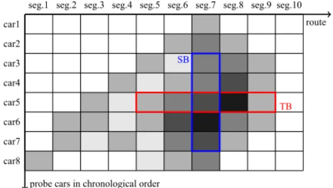
dðs;xÞ to calculate a degree of anomaly, denoted byD, and gives an alert when D exceeds a given threshold. We introduce alternative definitions forDbased on two different approaches, namely, a trajectory-based (TB) approach and a segment-based (SB) approach.Fig. 2shows an example of the two approaches.

TB approach: In this approach, the detection algorithm attempts to find the trajectory of a probe car whose behavior is abnormal. A probe car travels along a route, and we measure the divergence dðs;xÞfor each segment

route

probe cars in chronological order car8 car7 car6 car5 car4 car3 car2 car1

seg.1 seg.2 seg.3 seg.4 seg.5 seg.6 seg.7 seg.8 seg.9 seg.10

TB SB

Fig. 2.Example of trajectory-based (TB) and segment-based (SB)

approaches. The shades of gray indicate the value ofd, the degree of anomaly, which is calculated for each vehicle for each segment. The red rectangle is a sliding window used in the TB approach, and the blue rectangle is used in the SB approach. The length of the“TB”sliding window is constant, and the sum of thedvalues in the sliding window is evaluated to detect incidents. The length of the“SB”sliding window can vary in this view because the sliding window is defined using a time parameter, and the average of thedvalues in the sliding window is evaluated.

(7)

traversed. Assume thatdis a sequence of measureddðs;xÞ

values,N_dis the number of observations ind, anddiis the

i-th value ind. The oldest observation isd1, and the latest isdN_d. Because we have defineddðs;xÞto have the property of additivity so that the divergence of consecutive obser-vations can be quantified as the summation of the diver-gences for each observation, the divergence of the whole trajectory can be defined as follows:

D¼X

N_d

i¼1

di: ð27Þ

The more a car deviates from its usual behavior, the larger

Dwill be. However, ifDis defined as above, it will continue to increase as long as the car runs, and any trajectory would be determined eventually as being anomalous. Tak-ing an average over the whole trajectory can avoid this problem, but it is still a problem that the value for D

cannot be obtained until the probe car finishes traveling. It is also a problem that the sphere of influence of an incident cannot be specified. Therefore, we redefineDas the sum ofNconsecutive divergences:

D¼ X

i0þN1 i¼i0

di: ð28Þ

This version of D can be calculated in real time by maintainingdiusingN-length sliding windows and using its summation[9].

SB approach: In this approach, the detection algorithm monitors the divergences over time for each segment and gives an alert when the divergence is sufficiently high. Assume that several probe cars have passed through a segmentsfor the pastTseconds. The degree of anomaly

dðs;xÞcan be calculated for each observation, respectively. Let SWðs;TÞ be the set of d values. Then SW can be considered to be a sliding window over the timeT, which is drawn as a blue rectangle inFig. 2. Note thatjSWðs;TÞj, the cardinality of the set SW, is equivalent to the number of probe cars traversing the segment s for the past T

seconds, and can therefore vary according to the time. We now defineDas the sum ofdin SW:

D¼ X

dASWðs;TÞ

d: ð29Þ

However, this Dwill also increase as the traffic becomes dense, i.e., as the number of probe cars traversing the segment withinT seconds increases. We therefore revise the definition ofDto take an average over the probe cars in the sliding window:

D¼ 1

jSWðs;TÞj

X dASWðs;TÞ

d: ð30Þ

Whereas the TB approach tries to find abnormal behavior by a probe car, the SB approach is designed to simulate roadside-sensor-based traffic monitoring via probe-car data. A sliding window in the SB approach continuously watches a certain segment so that the detector can output the time and place of an incident.

4. Experiment

4.1. Dataset and preprocessing

Our PCD was obtained from probe cars traveling on the Shuto Expressway system during 2010 and 2011. The PCD include several tens of millions of observations. We first conducted data preprocessing, which comprised five phases: segment definition, map matching, trajectory identification, interpolation, and labeling. These proce-dures are described below.

Segment definition: As defined in Section 3.1, a certain segment corresponds to a certain 50-m length of roadway for a certain direction on a certain expressway route for a one-hour period regardless of the day. We defined the road segments by partitioning each route on the expressway every 50 m. The direction was noted. We also divided each day into 24 h and associated each segment with one-hour periods. This experiment did not consider days of the week.

Map matching: Although the above definition of a seg-ment is based on an expressway route, the location data in the PCD were described in terms of the two-dimensional coordinates of longitude and latitude, with the original observation not related to any particular segment. Map matching is a technology for identifying the road segment on which the vehicle is traveling and for locating the vehicle within that segment [45]. Several map matching methods have been proposed[46,47]. In this experiment, map match-ing was conducted in the simplest way: a probe car's observation was matched with the nearest segment to the car's location. The direction was estimated from the angular difference between the probe car's heading azimuth in the PCD and the segment's azimuth for each direction, and choosing the direction that gave the smaller angle. We used the National Land Numerical Information (NLNI)1 as the roadmap data. This set of data contains linestrings, which represent the shape of expressways and toll roads. The shape of junctions is not represented strictly, and road-width information is not included. After the map matching, we removed noisy records, namely, those more than 100 m from the nearest road. An observation was also removed if the angular difference between its heading azimuth and the segment's azimuth was more than 451.

Trajectory identification: To identify the continuous move-ment of the car, i.e., its trajectory, we grouped all observations in the dataset of records by anonymized car ID and sorted them by timestamp for each group, before concatenating them in chronological order whenever the time gap between two consecutive observations was 60 s or less.

Interpolation: We used a probe car's speed as the obs-erved value in this experiment. However, as mentioned in Section 3.3, our detection method estimated the current state for each trajectory for each segment that the car had traversed. Our 50-m segment was too short for fast-moving probe cars to provide observations for every segment, whereas a slow-moving car could generate multiple observa-tions in a single segment. Accordingly, we used the mean speed as the observation value for each segment for each

1

(8)

Table 2

Statistics for the dataset.

Route Direction Length

(km)

#in part (a)/(b)/(c)

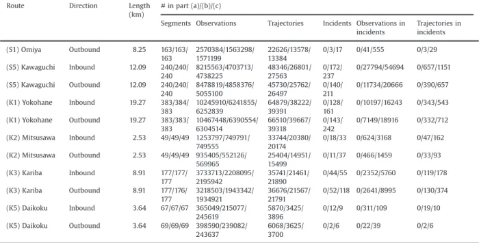
Segments Observations Trajectories Incidents Observations in incidents Trajectories in incidents (1) Ueno Inbound 4.30 85/85/85 792078/454175/ 511037 20985/11728/ 13568 0/11/22 0/310/633 0/39/74 (1) Haneda Inbound 12.58 250/250/ 250 6479136/3991898/ 3889471 74022/42323/ 43674 0/311/ 435 0/32234/44159 0/1273/1766 (1) Haneda Outbound 12.58 250/250/ 250 6246959/3788658/ 3665425 70453/40219/ 41482 0/116/ 203 0/9246/17460 0/440/779 (2) Meguro Inbound 5.70 112/112/ 112 1812270/1038831/ 954443 23782/13332/ 12260 0/71/98 0/2829/3468 0/166/185 (2) Meguro Outbound 5.70 112/112/ 112 1463662/872699/ 736948 17354/10280/ 8678 0/15/14 0/503/321 0/21/18 (3) Shibuya Inbound 11.70 232/232/ 232 9490711/5569544/ 5369891 65065/38621/ 38479 0/425/ 609 0/51908/74377 0/1640/2381 (3) Shibuya Outbound 11.70 233/233/ 233 8630888/5255259/ 5162198 62734/38563/ 39184 0/332/ 403 0/38110/51231 0/1103/1570 (4) Shinjuku Inbound 13.27 264/264/ 264 10681788/6252381/ 6093679 70500/40900/ 40431 0/394/ 514 0/68705/73368 0/2061/2215 (4) Shinjuku Outbound 13.27 264/264/ 264 10142665/6132584/ 5967115 68588/40519/ 39194 0/436/ 449 0/82656/71391 0/2093/1963 (5) Ikebukuro Inbound 21.10 420/420/ 420 17186588/9907871/ 9445068 110929/64056/ 62187 0/510/ 702 0/69114/115972 0/2354/3646 (5) Ikebukuro Outbound 21.10 420/420/ 420 16416424/9335481/ 9086078 103907/59799/ 58265 0/568/ 816 0/58386/114376 0/2120/3579 (6) Misato Inbound 10.23 203/203/ 203 6479441/3786663/ 3619748 44353/25326/ 24532 0/232/ 311 0/35096/62137 0/863/1369 (6) Misato Outbound 10.23 203/203/ 203 7015915/4090983/ 4006477 44909/26295/ 25354 0/137/ 144 0/15521/16618 0/464/607 (6) Mukojima Inbound 9.41 187/187/ 187 4944680/3102482/ 2611225 78108/46307/ 41934 0/226/ 274 0/17679/22290 0/927/1213 (6) Mukojima Outbound 9.41 187/187/ 187 6304960/3691151/ 3489748 78388/45684/ 43391 0/377/ 441 0/32256/45488 0/1452/1811 (7) Komatsugawa Inbound 11.19 222/222/ 222 4102884/2507305/ 2208502 39227/23071/ 20044 0/124/ 176 0/10309/12643 0/438/547 (7) Komatsugawa Outbound 11.19 222/222/ 222 4084778/2609988/ 2259405 29087/18868/ 16264 0/35/35 0/2142/3433 0/81/111 (9) Fukagawa Inbound 5.35 105/105/ 105 2427724/1327255/ 1362920 30616/16343/ 16780 0/93/178 0/4482/9070 0/243/436 (9) Fukagawa Outbound 5.35 105/105/ 105 1991012/1043268/ 1111541 24652/13135/ 13532 0/28/10 0/456/395 0/46/21 (11) Daiba Inbound 3.68 71/71/71 1505294/818800/ 837530 25453/13523/ 14222 0/94/158 0/3543/8010 0/220/428 (11) Daiba Outbound 3.68 72/72/72 2338885/1274658/ 1394220 34977/19043/ 20981 0/28/36 0/1384/1406 0/76/88

(C1) Inner circular Counterclockwise 14.00 278/278/ 278 10987711/6478632/ 6125324 228108/132148/ 127611 0/993/ 1181 0/59382/83258 0/3453/4710 (C1) Inner circular Clockwise 14.00 278/278/

278 11220562/6521415/ 6162208 212109/123424/ 117349 0/1038/ 1309 0/71823/86398 0/3380/3961 (C2) Central circular (west) Counterclockwise 10.79 214/214/ 214 4380668/3173120/ 3295236 39442/25426/ 25621 0/276/ 444 0/15142/27339 0/649/1139 (C2) Central circular (west) Clockwise 10.79 214/214/ 214 3340908/2735642/ 2973822 31195/22465/ 23639 0/235/ 350 0/13478/21081 0/597/946 (C2) Central circular (east) Counterclockwise 25.22 501/500/ 500 16248358/9138931/ 9122772 104236/59352/ 58779 0/480/ 592 0/75190/125806 0/2093/3245 (C2) Central circular (east) Clockwise 25.22 501/501/ 501 17636512/10035085/ 9935318 107118/61243/ 60511 0/577/ 745 0/51813/86449 0/1480/2224

(Y) Yaesu Northbound 1.55 30/30/30 193661/107788/

104587 7321/4057/ 3940 0/29/54 0/313/536 0/38/70 (B) Bayshore (west) Eastbound 37.91 755/755/ 755 19365358/11199556/ 11705000 84020/48877/ 51501 0/121/ 191 0/14131/25462 0/499/792 (B) Bayshore (west) Westbound 37.91 757/757/ 757 17326082/10325601/ 10673341 73703/41633/ 43200 0/121/ 156 0/8304/18252 0/263/533 (B) Bayshore (east) Eastbound 24.01 479/479/ 479 21959324/11994826/ 13071082 119437/64043/ 70639 0/262/ 499 0/32253/74072 0/1066/2075 (B) Bayshore (east) Westbound 24.01 479/479/ 479 23047168/12873257/ 13746786 121868/65826/ 72143 0/228/ 492 0/63681/142289 0/1505/3422 (S1) Omiya Inbound 8.25 163/163/ 163 2893492/1616952/ 1679369 25837/14486/ 14005 0/4/17 0/101/312 0/7/25

(9)

trajectory. This was obtained from the time required for the car to pass through the 50-m segment after we calculated the time when the car entered and left any segment by linear interpolation. Again, we removed noisy trajectories that traversed less than 10 segments, i.e., a 500-m distance.

Labeling: For the evaluation, we labeled each observa-tion in the trajectories, using the traffic log made available by the administrator of the Shuto Expressway. This traffic log was recorded via stationary sensors on or alongside the roads every five minutes, together with manual annota-tions about incidents such as accidents and construction. An observation was labeled as anomalous whenever the stationary sensor nearest to the segment recorded an incident at that time.

According to NLNI, the Shuto Expressway system comprises 29 routes, including short branches, and every route has traffic in both directions. Because the regulation and traffic patterns are different for each route, we partitioned our dataset to account for each direction on each route. We removed route data involving less than two actual incident occurrences. Because we did not have ground truth data for 2010, we conducted a cross-validation as follows. We first divided the data into three parts: (a) the data during 2010, (b) the data during the first half of 2011, and (c) the data during the second half of 2011. We then estimated the model using (a) beside either (b) or (c), with the detection test conducted using the remaining part. For the remainder of this paper, _“Fold 1_” denotes the trial with the training dataset (a) and (b), and

“Fold 2”denotes the trial with the training dataset (a) and (c). Table 2 summarizes the statistical information for our PCD after the preprocessing. In the remainder of this section, we estimated a traffic state model using a whole training dataset so that the traffic state“topic” was learned globally among

routes, whereas traffic incident detection was conducted independently for each route.

4.2. Parameter estimation

After the preprocessing, we estimated the parameters of our traffic state model for each training dataset. In this experiment, the observed values represented the speed of probe cars as nonnegative integers, and we assumed a Poisson distribution for the probability distribution corre-sponding to each traffic state. We implemented the EM algorithm described in Section 3.2 using OpenMP for multiprocessing. The estimation was executed on our 32-core Xeon computer.

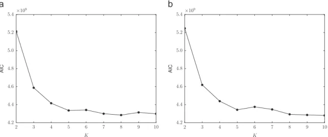
We first examined the optimal value ofK, the number of traffic states, using Akaike's information criterion (AIC). The optimal parameter value is that corresponding to the minimum AIC value, which means that the estimated model will achieve high likelihoods via a simple model, i. e., a model having few parameters.Fig. 3shows the plots of the AIC for different values of K. The effect of model complexity was substantially less than that of the like-lihood for improving the AIC, with the AIC value being almost the same for largeK. We therefore assumed a value forKof 8 when conducting the experiment.Fig. 4shows the log-likelihood of the model against the number of iterations of the EM algorithm, up to 20 iterations. In this experiment, we considered the algorithm to have con-verged when the improvement in log-likelihood fell below 0.01%, which was achieved after seven iterations. The execution of the EM algorithm up to the seventh iteration required about 18 min for both folds.

Table 2(continued)

Route Direction Length

(km)

#in part (a)/(b)/(c)

Segments Observations Trajectories Incidents Observations in incidents Trajectories in incidents (S1) Omiya Outbound 8.25 163/163/ 163 2570384/1563298/ 1571199 22626/13578/ 13384 0/3/17 0/41/555 0/3/29 (S5) Kawaguchi Inbound 12.09 240/240/ 240 8215563/4703713/ 4738225 48346/26801/ 27563 0/172/ 237 0/27794/54694 0/657/1151 (S5) Kawaguchi Outbound 12.09 240/240/ 240 8478819/4858376/ 5055100 45730/25762/ 26497 0/140/ 211 0/11734/20666 0/390/657 (K1) Yokohane Inbound 19.27 383/384/ 383 10245910/6241855/ 6252839 64879/38222/ 39391 0/128/ 161 0/10197/16243 0/343/543 (K1) Yokohane Outbound 19.27 383/383/ 383 10467448/6390554/ 6304514 66510/39667/ 39318 0/143/ 242 0/7149/18916 0/332/712 (K2) Mitsusawa Inbound 2.53 49/49/49 1253797/749791/ 749555 33744/20380/ 20174 0/18/33 0/624/3168 0/47/162 (K2) Mitsusawa Outbound 2.53 49/49/49 935405/552126/ 569965 25404/14951/ 15499 0/11/37 0/466/1459 0/33/93 (K3) Kariba Inbound 8.91 177/177/ 177 3733713/2208095/ 2195942 35741/21461/ 21890 0/44/55 0/2352/5760 0/119/178 (K3) Kariba Outbound 8.91 177/176/ 177 3218503/1943342/ 1934921 36676/21567/ 21791 0/52/118 0/2641/8995 0/130/374 (K5) Daikoku Inbound 3.64 67/67/67 365049/215077/ 245619 5870/3425/ 3896 0/12/9 0/311/109 0/19/10 (K5) Daikoku Outbound 3.64 69/69/69 398590/239082/ 243637 6068/3625/ 3700 0/2/6 0/22/39 0/2/6

In some cases, additional segments were recognized because the shape information of the roadmap data we used is incomplete at junctions. The nonexistent segments were rarely recognized by the map-matching process.

(10)

Fig. 5shows the actual histogram for a segment of the inbound Shibuya route as a stepwise line chart and the estimated Poisson mixture as a solid curved line. Each of the eight Poisson distributions was multiplied by the mixing coefficients

π

sk, which are also shown in Fig. 5 as dashed curves. We note that the estimated curve almost fits the actual histogram for the training dataset.

Fig. 6shows the usual traffic state

σ

ðsÞfor each segment in the Shuto Expressway system, which was estimated using the learned traffic state model. The color of the segment indicates the parameter value for the Poisson distribution of

σ

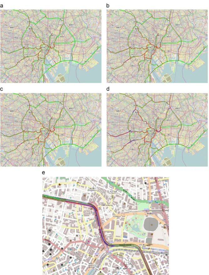
ðsÞ, i.e., the mean speed in the usual traffic state. Green represents high speed (100 km/h), red is moderate speed (50 km/h), and blue is

“almost stopped”(0 km/h). The four figures (a)–(d) show the usual traffic over four different one-hour periods. We can see that the traffic is usually slow at several places during the rush hour, indicating that congestion usually occurs, whereas the traffic is almost smooth during the day and at midnight.Fig. 6(e) shows an enlarged view near the Iidabashi interchange on the

Fig. 3.Plot of AIC for different values ofK, the number of traffic states: (a) Fold 1 and (b) Fold 2.

Fig. 4.Log-likelihood of the model against the number of the EM iterations, whereKis 8: (a) Fold 1 and (b) Fold 2.

Fig. 5.Histogram of the speed of probe cars in a segment and the

(11)

Fig. 6.Estimated usual traffic stateσðsÞfor all 50-m segments, drawn on the OpenStreetMap. The color of a segment indicates the parameter value for the Poisson distribution of the maximum probable state, i.e., the mean speed ofσðsÞ. Green represents high speed (100 km/h), red is moderate speed (50 km/h), and blue is“almost stopped”(0 km/h) (map tiles © OpenStreetMap contributors, CC BY-SA 2.0). (a) 00:00–01:00, (b) 07:00–08:00, (c) 13:00–14:00, (d) 18:00–19:00 and (e) 18:00–19:00 near the Iidabashi interchange on the Ikebukuro Route.

(12)

Ikebukuro Route between 18:00 and 19:00. The outbound direction is from the lower right to the upper left.2_{The figure}

shows that outbound traffic is usually slow near sharp curves and at the Iidabashi entrance in the center of the map, whereas the usual state of the other segments, including the inbound route, is“moderate”or“smooth.”Here, it can be seen that the estimated traffic state model has enabled any road section during a certain period to be characterized using a single set of traffic states, with the usual pattern of traffic thereby being described at a fine level of time and space granularity.

4.3. Incident detection

Using the estimated traffic model, we evaluated the performance of the proposed method. Our detection method gives an alert when the divergence of an input set of observation values for the estimated traffic model exceeds a given threshold. We regarded a set that includes at least one value labeled as an anomaly to be a truly anomalous set. The two proposed algorithms require parametersNorT.Table 3 summarizes the parameter values used in this experiment.

The results shown in Section 4.2 indicated that the traffic pattern was different for each route, section, and time, and therefore the detection threshold must be changed accordingly. Although the granularity of such a threshold tuning should depend on the amount of data, we know of no method to determine the appropriate granu-larity. In this experiment, we conducted incident detection for each route, because the traffic characteristics were considered to be comparatively homogeneous on an indi-vidual route. We evaluate the selectivity performance of incident detectors in terms of a receiver-operating char-acteristic (ROC) curve. An ROC curve is drawn by plotting the true positive rate (TPR) against the false positive rate (FPR) at any threshold. Both TPR and FPR change according to the detection threshold: both values are zero when the threshold is high enough not to give an alert for any input, whereas they are equal to one when the threshold is low enough. With an ideal detector, TPR can be one with FPR being zero at a certain threshold. Therefore, the “area under the curve”(AUC) reflects the discrimination perfor-mance, with larger AUC values indicating better discrimi-nation. For each route, we first applied the detection algorithms to our twofold dataset and obtained the values of divergence for each input. We therefore have possible values for the threshold at which either TPR or FPR changes. The ROC curve was drawn by plotting TPR against FPR in all cases.

We conducted a comprehensive experiment. The detec-tion performance was examined by calculating AUC values

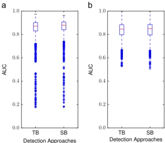
respectively for all combinations of the algorithm (TB or SB), parameters (shown inTable 3), divergence function (proposed inSection 3.3.1), and route. At the beginning of the analysis of results, we first investigated the perfor-mance of the two algorithms proposed in Section 3.3.2. Fig. 7 shows box plots for the distribution of the AUC values, comparing the TB and SB approaches. Values less thanQ11:5IQR are plotted as outliers, whereQ1 is the first quartile and IQR is the interquartile range, the difference between the first and third quartiles. As seen inFig. 7, there is no significant difference between the TB and SB algorithms' performance. Therefore, we decided to examine the performance further only in terms of the TB algorithm.

Next, we investigated the performance of the diver-gence functions proposed inSection 3.3.1.Fig. 8shows the results in terms of box plots similar to those above. The results indicate that the weighted KL divergence, defined as Eq. (23), achieved the best performance among the functions because its AUC values were the most concen-trated at high values and its the median was the highest. Therefore, we used this function for the remainder of the experiment.

We also examined the optimal value for the parameterN, the length of the sliding window, using weighted KL diver-gence as the diverdiver-gence function.Fig. 9shows the distribution of AUC values for eachN. From this figure, the discrimination performance was almost unchanged asNincreased.Fig. 10 shows the ROC curves for four cases whenNwas 10. Because we were using 50-m segments, the length of the sliding window was equivalent to a 500-m distance along a route.

As shown inFig. 9, the AUC value was more than 0.8 in most cases. The best performance was achieved on the northbound Yaesu route, and the second best case was the outbound Kawaguchi route. The TPR reached 80%, with the FPR being less than about 3% in both cases, as shown inFig. 10 (a) and (b). On the other hand, there were a couple of outlier Table 3

Tested parameter values.

Detection algorithm Parameter values

TB N¼1, 2, 3, 4, 5, 10, 15, 20, 25, 30

SB T¼60, 300, 600, 1800, 3600

Fig. 7.Box plots of the AUC values for the proposed TB and SB methods.

Each box plot describes the distribution of AUC values for all combina-tions of the parameters, divergence function, and route: (a) Fold 1 and (b) Fold 2.

2

(13)

cases where the discrimination performance was extremely low. The worst case was the outbound Daikoku route, as shown inFig. 10(c). The dataset for this route contains a very small number of actual incidents. Therefore, the detection performance through the dataset is greatly influenced by the characteristics of individual incidents. We investigated the dataset in detail, and we found trajectories that look as if the traveling behavior is different from the usual because of noise, whereas there was actually no incident at that time. The proposed method detected them as anomalies, and such misdetections influenced the detection performance evalu-ated by the ROC curves. The second worst case was the outbound Meguro route. After the TPR reached 40%, with the FPR being less than 1%, the ROC curve continued almost

straight ahead to the upper right corner. From the dataset for this route, the proposed method could detect incidents with high precision when the threshold was high enough. When the threshold was decreased, the method detected other segments near incident-labeled segments as well as the abnormal segments.

4.4. Comparison with a previous method

So far, we have reported on the performance of the pro-posed method and obtained the best parameters and func-tions. We also conducted an experiment to compare our method with a baseline method, namely, the method of Zhu et al. [25], which was described in Section 2. The latter

Fig. 8.Box plots of AUC values for the TB algorithm for each divergence function: (a) Fold 1 and (b) Fold 2.

Fig. 9. Box plots of AUC values for the TB algorithm with the weighted KL divergence function for eachN, namely, the number of consecutive segments in a

(14)

method finds traffic incidents by applying a distance-based outlier detection algorithm to feature vectors, which are carefully extracted using heuristics and normalized according to the mean and variance. The algorithm calculates the distance between any two feature vectors and detects outliers whenever the average distance of a vector to any other point is more than a given threshold. This algorithm runs in a batch manner, and its complexity isOðN2_Þ_{, where}_N_{is the number}

of observed feature vectors.

In this paper, we have tackled the problem of detecting traffic incidents in real time. We modified the baseline method to enable its application to our dataset in a streaming manner as follows. First, a queue was prepared to store the lastnfeature vectors. Variables for storing the sum and sum of squares of feature vectors for each dimension were also prepared, to enable the mean and variances to be calculated. Whenever a vehicular speed is observed, a feature vector is generated using both those data and data observed in the past, with the sum and sum of squares being updated. Any vectors in the queue in addition to the input vector are then normalized according to the mean and variance for each dimension before the distances between the input feature vector and any vectors in the queue are calculated. The

algorithm outputs the average distance as the degree of anomaly for the input vector and detects whether it exceeds a given threshold. Then, if the queue is full, the oldest vector is removed, and the sum and the sum of squares are updated. Finally, the input vector is queued. We can infer that the detection performance is improved as the queue length n

increases because the detector can then exploit more knowl-edge in determining anomalies. However, the algorithm will take longer time to execute because the computational complexity isO(n) for each input, which might prevent the algorithm from working in real time.

We compared the baseline and proposed methods for three routes that were carefully selected. The chosen routes were the clockwise Inner circular route (Route C1), represent-ing a slow-traffic rrepresent-ing road, the outbound Ikebukuro route (Route 5), representing a moderate-traffic radial road, and the eastbound Bayshore (east) route (Route B), representing a fast-traffic road. We implemented the baseline method using OpenMP to enable parallel execution with up to 32 threads.3

Fig. 10.Detection performances of the proposed method in terms of ROC curves. (a) The best case: the northbound Yaesu route, (b) the second best case:

the outbound Kawaguchi route, (c) the worst case: the outbound Daikoku route and (d) the second worst case: the outbound Meguro route.

3

Our proposed detector was implemented without involving parallel-processing technologies.

(15)

Varying the queue length from 1 to 500,000, we executed the base line method with a single thread to reduce the overhead of context switching whenever the queue length was less than 10,000. Elsewhere, we used 32 threads to reduce the actual time of execution. We evaluated the two methods in terms of their AUC values and CPU times.

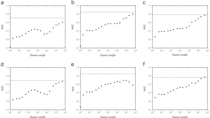
Although it was suggested [25] that input instances should be filtered in accordance with the heuristic condi-tions, we first evaluated the performance of the baseline method without any filtering to compare its discrimination performance for each input with that of the proposed method. The performance was evaluated using AUC values. Figs. 11 and 12 show the performance of the filterless baseline method with various queue lengths, in terms of the AUC values and the CPU time required to process the input dataset, with the horizontal dashed line showing the performance of the proposed method. Our method com-pleted the detection task for a half year within 100 s for each route. As indicated in the figures, the performance of the baseline method was improved as the queue length increased because it could utilize a wider range of knowl-edge, but at a considerable cost in time to complete the detection. The detection performance of the proposed method was comparable to that of the baseline method when the queue length is 500,000, but the CPU time for our method was less than 0.1% of that for the baseline. Although the detection performance of the baseline method could be improved with a larger queue length to exploit more data, the algorithm would take much longer than would our method, thereby causing difficulty for real-time applica-tions. Our method has access to data observed in the past in a compact form and can detect incidents in a short time.

Next, we evaluated the performance of the baseline method using the proposed filtering [25], to compare the detection performance for each incident with that of the pro-posed method. The filter discards any input vectors consid-ered not to be from an incident, based on heuristics. Although the ROC curve should connect points (0,0) and (1,1), the baseline method with filtering broke off before the (1,1) point was reached, because the method filtered out some feature vectors of incidents, with the number of tested trajectories being less than the total number of trajectories. From the perspective of incident detection, dropping input vectors that are actually from an incident is permissible provided that at least one input vector is detected for the incident. We therefore evaluated the performance using the detection rate (DR), the ratio of the number of detected incidents to that of actual incidents. Because several trajec-tories may be involved in one incident, we judged that an incident was correctly detected if at least one trajectory or feature vector was detected by each method.

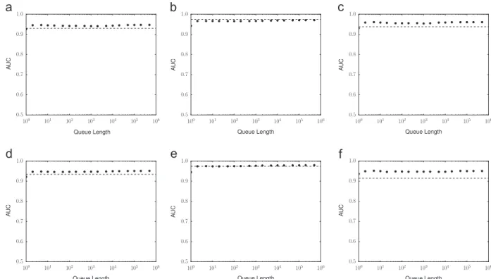
As with the ROC curve, the FAR–DR curve is drawn by plotting the DR against the FPR at various threshold. We used the AUC value of the FAR–DR curve instead of the ROC curve, which we call the DR-AUC value in this paper. Because the FAR–DR curve of the baseline method also broke off before (1,1) was reached, the DR-AUC value was calculated by linear interpolation between the right-hand end of the FAR–DR curve and (1,1).Fig. 13shows the DR-AUC values for the filtered baseline method with various queue lengths, andFig. 14shows the CPU times required to process the entire input dataset. From these figures, the detection performance of the proposed method was com-parable to that of the baseline method.

Fig. 11.AUC values for the filterless baseline method with various queue lengths. The horizontal dashed line shows the AUC values for the proposed

(16)

5. Discussion

Previous work has exploited several heuristics to detect traffic incidents and congestion, whereas our work takes a completely statistical approach that avoids heuristics and enables real-time applications. In this study, we introduced a traffic state model based on a probabilistic topic model, proposed an incident detection method using the model, and tested its discrimination performance and incident detection performance.

We found that the proposed method could detect incidents at the same level as the existing method in a shorter time. Because our method is generic and exten-sible, it would be expected to outperform existing meth-ods by including several heuristics that consider the context of individual situations. For example, it would be effective to optimize the detection threshold according to the section and time. Whereas the experiment in this paper took only the route into account, the granularity of threshold tuning remains to be determined in future studies. Although we used only the vehicular speed as the observed value in this experiment, other features, which can be extracted carefully from PCD via heuristics, should also contribute to improving the detection perfor-mance. In addition, it might be effective to extend the traffic state model by introducing other latent variables and relations among them. It is also possible to apply our method to data obtained by roadside sensors, given that a road segment in our model can correspond to a stationary sensor. Again, this might improve the detection

performance. In that case, we could employ the detection algorithm for the SB approach instead of using the TB ver-sion. Although we evaluated the detection performance using ROC curves, determining the value of the threshold is necessary for practical use. It is known that the detec-tion threshold can be optimized using ROC curves [48]. The adaptive optimization of detection thresholds was not considered here, being left to future work.

From the perspective of continuous traffic monitoring, any incident should be followed up from its occurrence to its resolution. Although it is sufficient for the initial detection of an incident that at least one input instance can be detected reliably, even if other instances of the incident are not detected, this would be insufficient for these applications. To realize an automated monitoring system, it must be able to determine correctly whether a current observation of traffic or a trajectory is anomalous.

We found that the proposed method could distinguish trajectories that were involved in an incident better than the existing method. The Shuto Expressway system has many bottlenecks, such as curves and narrow sections that require frequent changes in vehicular speed, unlike straight freeways. We speculate that this is the reason that our intuitive method found that _“unusual_” car behavior worked better than a heuristic method that pays attention to changes in speed. As our method detected nonabnormal segments near places of incidents as well as abnormal segments in the experiment, future work should elaborate the algorithm so that the detector can have high resolution of discrimination. Future work should also verify that this approach is also effective for

Fig. 12.CPU times for the filterless baseline method with various queue lengths. The horizontal dashed line shows the CPU time for the proposed method:

(17)

local streets where normal behavior involves cars stopping frequently.

We tested the performance of the proposed method using several of the divergence functions proposed in

Section 3.3.1and found that using the negative log prob-ability of the observation as the divergence function was the worst performer. This observation indicates that for incident detection problems, it is not satisfactory simply to

Fig. 13.DR-AUC values for the filtered baseline method with various queue lengths. The horizontal dashed line shows the DR-AUC value for the proposed

method: (a) Route C1, Fold 1, (b) Route 5, Fold 1, (c) Route B, Fold 1, (d) Route C1, Fold 2, (e) Route 5, Fold 2, and (f) Route B, Fold 2.

Fig. 14.CPU times for the filtered baseline method with various queue lengths. The horizontal dashed line shows the CPU time for the proposed method:

(18)

find low-probability objects. Conversely, the experiment showed that KL divergence was the best performer for the divergence function. In our model, a traffic state is asso-ciated with a Poisson distribution, which generates an observation value for vehicular speed. As shown in the Appendix to this paper, given two Poisson distributionsp1 and p2 whose parameters are

λ

1 and

λ

2 respectively, KLðp1Jp2Þ4KLðp2Jp1Þ holds where

λ

14

λ

240. Because

the parameter of the Poisson distribution is equivalent to its mean, this property can be interpreted in the context of our traffic state model as follows. Assume a fast traffic stateFwhose mean speed is

λ

F and a slow traffic stateS whose mean speed is

λ

S, where

λ

F4

λ

S. According to the property of KL divergence, the divergence of the current traffic stateSfrom the usual traffic stateFis greater than that of the current traffic stateFfrom the usual traffic state

S. This property is advantageous for the incident detection problem because traffic incidents often cause traffic con-gestion and a slowdown. However, a particular incident will be hard to detect by the proposed method if the traffic behavior in the incident is very similar to regular sponta-neous congestion. It remains a challenge for future research to detect these kinds of incidents and to extract a deeper insight about each detected incident, which might involve an accident, car troubles, or road debris.

So far, we have discussed the discrimination and detection performance of the proposed method. We now consider another topic of key interest, namely, real-time processing. Our detection method itself is scalable because its complexity isO(K) for each input, and the number of traffic statesKis not very large in practice, as shown in the experiment. We have designed and developed a real-time traffic incident detection system, which applies our algorithm to a PCD stream and shows the high-divergence segments on a map[9]. However, our detection method is based on the traffic state model, which was acquired via batch processing. In the long term, the usual pattern of traffic can vary, and it will be necessary to update the model by some means. For our experiment, the learning process for about 18 months of data was completed in about 18 min using parallel-processing technology, which suggests that regular updating might be a simple solution to this problem. Although our experiment showed that the number of traffic states was not very large in practice, the number of segments and observations will surely become greater in the future. This requires that the algorithm should be scalable in this respect. Further work is in progress to develop a scalable method for learning the model.

6. Conclusion

In this paper, we have studied the problem of detecting traffic incidents using PCD. Although congestion can be detected by monitoring vehicular speeds, it is a chronic condition in some spots and does not necessarily indicate the occurrence of an incident. To detect traffic incidents, we took an approach that identifies any unusual events. We first introduced a probabilistic topic model to describe the state of monitored traffic so that usual traffic behavior can be learned. We then proposed several divergence functions for evaluating the difference between the current and usual traffic based on the model and streaming algorithms to detect

high-diver-gence segments in real time. Our method was applied to real PCD collected for the entire Shuto Expressway system in Tokyo, and the discrimination and detection performance was evaluated. The results showed that our method could dis-criminate trajectories affected by incidents from other trajec-tories, using KL divergence as the divergence function, which enables monitoring of an incident from beginning to end.

Acknowledgment

This work was supported by the CPS-IIP Project in the research promotion program for national-level challenges

“Research and development for the realization of next-generation IT platforms” of the Ministry of Education, Culture, Sports, Science and Technology, Japan. The Nat-ional Land Numerical Information was provided by the Ministry of Land, Infrastructure, Transport and Tourism, Japan. The traffic log used in our experiment as the ground truth for incident occurrence was made available by Metropolitan Expressway Co., Ltd.

Appendix A. KL divergence between two Poisson distributions

The Poisson distribution is defined as follows: