Quantile combination for the EEM Wind Power Forecasting Competition

Quantile Combination for the EEM20 Wind Power

Forecasting Competition

Jethro Browell, Ciaran Gilbert, Rosemary Tawn and Leo May

University of Strathclyde Glasgow, UK

Email: [email protected]

Abstract—Combining forecasts is an established strategy for improving predictions and is employed here to produce proba-bilistic forecasts of regional wind power production in Sweden, finishing in second place in the EEM20 Wind Power Forecasting Competition. We combine quantile forecasts from two models with different characteristics: a ‘discrete’ tree-based model and ‘smooth’ generalised additive model. Quantiles are combined via linear weighting and the resulting combination is superior than both constituent forecasts in all four regions considered.

I. INTRODUCTION

This competition, hosted by the European Energy Markets (EEM) conference, was devised to promote improvements in wind energy forecasting to address some of the challenges introduced by increasing wind energy capacity. The competi-tion was focused on producing probabilistic day ahead wind energy forecasts for the four price regions of Sweden, in which a majority of energy is procured day ahead through the power exchange Nordpool. The price regions exist due to transmission constraints limiting liquidity and creating geographically unique supply and demand constraints. The price regions are also stratified roughly north to south, meaning that as well as experiencing differing mesoscale weather phenomena, each region’s wind power assets operate under distinct temperature climatology resulting in phenomena such as blade icing in some regions. The forecasting challenge is further compounded by increasing installed capacity in all four regions, thereby introducing a time varying scale factor in the historical wind energy production training data set.

Wind power forecasting has developed in parallel with the wider wind industry driven by the needs of market participants and power system operators, review extensively in [1]. While wind power forecasting is relatively mature and many commercial offerings exist today, research is ongoing to improve accuracy and forecast further ahead [2]. Notably, recent advances have come from incorporating new sources of data, such as girds of Numerical Weather Predictions (NWP) [3], turbine-level data [4], remote sensing [5], [6], and advances in NWP [7], enabled by contemporary data science. Wind power forecasting competitions are common in indus-try, where forecast-users often run trials of forecast services to compare skill and other qualities. In the academic sphere they provide an invaluable test bed for forecasting methods

by providing standardised datasets and evaluation protocols, minimising the possibility of cheating, and publishing the approaches of winning entries. The 14th edition of this confer-ence featured a wind power forecasting competition [8], and two editions of the Global Energy Forecasting Competition have included wind power [9], [10], where tree-based methods emerged as leading methodologies. However, the present com-petition has a number of novel features: forecasting regional production rather than individual wind farms, provision of gridded NWP, and provision of ensemble NWP. We discuss these aspects in mode detail in Section V.

The competition set-up and data are detailed in Section II, followed by descriptions of the forecast methodologies we employed in Section III. Section IV presents our results, while Section V concludes with a discussion of our learning and reflections on the competition and performance of our forecasts.

II. COMPETITIONSET-UP

The competition required nine quantile forecasts (0.1,...,0.9) of total wind power production to be produced at hourly reso-lution for the four price regions of the Swedish electricity mar-ket. Gridded ensemble NWP covering Sweden were supplied, along with the details of wind farm capacity and location, and power production. The NWP comprised of forecasts for each hour of the day issued at 0600UTC the day before, so available in time to inform trading in European day-ahead electricity markets. All competition data and code is available with this paper, see the Acknowledgment section for details.

One year of training data was supplied, and the competition ‘tasks’ involved producing forecasts for the following two months given NWP. After each task, the actual power was released along with the NWP for the next task, effectively increasing the volume of training data by two months.

Quantile forecasts for each task were evaluated using the Pinball Loss function, given by

ρα,t(y (α) t , yt) =    αyt−y (α) t if yt≥y (α) t (1−α)y_t(α)−yt if yt<ty(α) (1) for a single price region, and averaged across timet, quantiles

α, and price regions (not indexed above). The average of the lowest five values from the six tasks gave the final score for each participant.

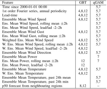
TABLE I

LIST OF FEATURES ENGINEERED FROM ENSEMBLENWPINPUT AND VERSIONS OF THEGBTANDBGAMMODELS THAT USED THEM. ALL CALCULATED FOR EACH PRICE REGION SEPARATELY TAKING THE MEAN

VALUE FORNWPGRID POINT CLOSEST TO EACH WIND FARM. ‘WEIGHTED’TO WEIGHTING BY INSTALLED CAPACITY. ‘POWER’WAS

ESTIMATED AT EACHNWPPOINT BASED ON HUB HEIGHT AND INSTALLED CAPACITY OF WIND FARMS USING EXPONENTIAL WIND SHEER

AND A SMOOTHED GENERIC WIND TURBINE POWER CURVE.

Feature GBT qGAM

Time since 2000-01-01 00:00 5,7 1st order Fourier series, annual periodicity 4,8,12 5,7

Lead-time 4,8,12 5,7

Ensemble Mean Wind Speed 4,8,12 5,7 Ens. Mean Wind Speed, rolling mean±2h 5,7 Ens. Mean Wind Speed, lead/lad -2–2h 5,7 Ensemble Mean Wind Gust 4,8,12 5,7 Ens. Mean Wind Gust, rolling mean±2h 5,7 Weighted Ens. Mean Wind Speed 4,8,12 5,7 W. Ens. Mean Wind Speed, rolling mean±2h 4,8,12 5,7 W. Ens. Mean Wind Speed, lead/lad -2–2h 4,8,12 Ensemble Mean Wind Direction 4,8,12 5,7

Ensemble Mean Power 7

Ens. Mean Power, rolling mean±2h 12 7 Ens. Mean Power, lead/lad -2–2h 12

Ensemble Mean Temperature 4,8,12 5,7 W. Ens. Mean Temperature 4,8,12 Ensemble Mean Temperature, past 24h mean 5,7 Ensemble Mean Temperature, past 24h min 5,7 p50 forecast from neighbouring regions 8,12 –

III. METHODOLOGY

The quantile forecasts are calculated through quantile re-gression, a supervised learning framework which minimised the loss function given in 1, wherein inputs comprise of features derived from NWP forecasts and power production is the target variable. These quantile models represent cut points in the conditional probability distribution of the target variable as functions of the forecast inputs. Applying these models to new input data yields a forecast of the conditional probability distribution of the target variable, which can aid decision making under uncertainty.

Estimating quantile regression models is typically iterative, minimising 1 through one or a combination of numerical methods. Because the efficiency of the numerical methods is related to the correlation between the target variable and the forecast inputs, a process of input or ‘feature’ engineering is undertaken to create features which represent physical phenomena which have greater explanatory power for the target variable than the raw forecast inputs. The list of features we considered in our models is in Table I. We take inspiration from the features used in [11], with the addition of temperature effects to capture blade icing.

In order to prevent overfitting when tuning the hyper-parameters of the quantile models, a process of stratifiedk-fold cross-validation was implemented. The average performance gives an estimate of out of sample performance of the selected hyperparameters, which are optimised via grid search. In this work the training data is divided into three folds with each month split into the three folds. This approach is not only convenient to implement but avoids clustering seasonal

0 1 2 3 2000−01 2000−07 2001−01 2001−07 Date (yyyy−mm) Maxim um P o w er (GW) Version Capacity Data Manual Modification Rolling Max Power

Price_region SE1 SE2

Fig. 1. Capacities for regions SE1 and SE2 for Task 6 based on the competition-supplied list of wind installations, a manually modified version of this list, and the rolling maximum of the recorded power production.

weather variations within any fold.

To address the changing installed wind capacity, we nor-malised each region’s measured power by the estimated ca-pacity so that it was in the range[0,1]. However, we observe that the capacity data provided is imperfect as not all wind farms appear to come online with their full capacity on the data listed. We therefore made a number of manual corrections to the installation data of some large wind farms (in order to retain spatial information) and to region totals based on measured power from available training data for each task. The effect of this can be seen in Figure 1. When large changes in capacity occurred during test period we smoothed these changes, as illustrated at SE1 in Figure 1.

In the subsequent subsections we describe the methods used to generate the task forecasts, including the two quantile regression techniques and the method of quantile combination. A. Gradient Boosted Trees

Gradient Boosting Trees (GBTs) are an ensemble of weakly predictive regression trees, combined to generate a powerfully predictive collective [12]. For each tree in the ensemble, the available input space is split into disjoint regions, where each observation is assigned to a ‘leaf’ of the tree. This allows for the capture of non-linear relationships, which is particularly suitable to the wind forecasting power curve [3], [11], [13]. Each tree is consecutively fit to the the negative gradient of the loss function, with respect to the entire ensemble so far, and that learning relationship is governed by important hyperparameters, such as the number of trees, the number of splits in a single tree (i.e. the depth of each tree), and a shrinkage factor which penalises the importance of each tree [14].

An important advantage of the GBT algorithm is that the loss function is flexible, and for this competition is used to directly minimise the quantile loss over the desired set of

nominal probabilities. For a pool of explanatory variablesxt=

(x1, x2, . . .)>, a regression tree is defined as fn =h(x;θn), which is specified by a vector of tree parameters θn, and the gradient boosting treeFN(xt)is an ensemble ofN regression trees. For target variabley, the ensemble predictor is

yt=FN(xt) +t= N

X

n=0

fn(xt) +t (2) wheref0(xt)is the initialisation guess andtis an error term. The ensemble of trees is constructed sequentially by estimating the latest via

argmin

fn

X

t

L(yt, Fn−1(xt) +fn(xt)) (3) for some loss function (i.e. quantile loss here) L(·). The negative gradient gn(x)is defined as

gn(xt) =− _∂L(y t, Fn(xt)) ∂Fn(xt) Fn(x)=Fn−1(x) , (4) and the regression tree is efficiently fit to this negative gradient by least squares θn= argmin θ X t [gn(xt)−h(xt;θ)] 2 . (5)

The ensemble is then updated with

Fn(xt) =Fn−1(xt) +λρnh(xt;θn) (6) where λ which is a user defined regularisation lever termed shrinkage, and ρn updates the tree predictions to match the general loss function

ρn = argmin ρ

X

t

L(yt, Fn(xt) +ρh(xt;θn)) . (7) The model fitting optimisation strategy is then based on two stages: least squares fitting of the base learner, i.e. a regression tree, followed by the parameter optimisation according to the general loss function via ρn [15]; ρn is computed separately for each terminal leaf for regression trees.

The shrinkage and tree depth hyper-parameters are selected for each region individually, usingk-fold cross validation and a grid search of the parameter space. The number of trees is kept constant at 1000, as is the minimum number of observations in each terminal node at 30, and the bag fraction at 90%.

Although this algorithm has intrinsic feature selection capa-bility, different model formulations were also tested carefully. This is because empirically it is often found that variables that are used even sparingly in the model fitting process can degrade forecast skill. For instance, higher skill was found by excluding the individual wind speed ensemble members, when using the ensemble average features. Therefore, we built up the input variable space comparing improvements against a parsimonious model. A final quick feature selection stage is also used on the final model formulation, i.e. model 12 in Table I, by thresholding the feature importance in sparse models for the 0.1, 0.5, and 0.9 quantiles, which improved the forecast skill in three out of the four price regions.

B. Boosted Generalised Additive Models

Generalised additive models (GAMs) are a flexible gener-alisation of linear models of the form

g(yt) =Atθ+ X i fi(xi,t) + X j fj(xj1,t, xj2,t) (8)

where At is taken from row t of the design matrix X and includes columns for which linear terms are included in the GAM, with corresponding parametersθ;g(·)is a link function or transformation as in Generalised Linear Models; and f(·)

are smooth function of uni- or bivariate inputs fromX [16]. These ‘smooths’ are forms as linear combinations of basis functions f(x) = K X k=1 bk(x)βk (9)

where, in the present study the basis functionsbk(·)are from the P-spline basis.

Given the large number of parameters in a typical GAM, parameter estimation can be challenging and regularisation is advisable to ensure that smooths are only as ‘wiggly’ as necessary and no more. In this work, we estimate quan-tile regression GAMs (qGAM) via component-wise gradient boosting, which has a similar effect as optimising a penalised loss function [12], [17].

For the EEM competition, we estimated one qGAM model for each quantile0.1, ...,0.9and price region using the features listed in Table I. The first three were included as linear terms to capture long-term trends and seasonality, with univariate smooths of all others included where the relationship with power is known to be non-linear, plus a bi-variate smooth of lead-time and ensemble mean wind speed. Version 5 was used for all six tasks and version 7 was used from task 2 onward. For each task, forecasts from the best performing GAM were combined with the best performing GBT, as described in the next section.

C. Quantile Combination

It has been shown that a combination of different forecasts generally tends to outperform the individual forecasts, even where the combination is a straightforward average [18]. A simple approach using only one parameter (when two forecasts are combined) is the linear opinion pool, where a fixed weight is applied to each forecast and the weights are constrained to sum to one. In the case of the competition forecasts, we noticed that the relative performance of the two models varied across the quantiles, with the qGAM performing better than GBT towards the tails, and GBT better in the middle of the distribution. As such, we applied a linear combination where the weightw(α) _{was allowed to vary for each quantile}

y_t,(α_comb) =w(α)y_t,(α_GBT) + (1−w(α))y_t,(α_qGAM) . (10) We select w(α) _{through a grid search for each price region} and quantile, picking the weight that minimised the pinball loss based on the cross validation framework described above.

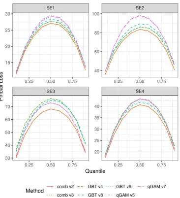
SE3 SE4 SE1 SE2 0.25 0.50 0.75 0.25 0.50 0.75 0.25 0.50 0.75 0.25 0.50 0.75 40 60 80 100 20 25 30 35 40 15 20 25 30 30 40 50 60 70 Quantile Pinball Loss Method comb v2 comb v3 GBT v4 GBT v8 GBT v9 qGAM v5 qGAM v7

Fig. 2. Cross-validation results for Task 6. The only difference between the combination version 4 and 5 is the use of GBT v8 rather than v12 in SE4. The year 2000 was the initial training data, and 2001 was split into six two-month tasks.

IV. COMPETITIONTASKS ANDRESULTS

The competition comprised of six tasks, with new training data available for each. This allowed for models to be re-trained with a larger volume of data in latter tasks, and importantly, for estimates of installed capacity to be updated. During the competition we made a number of manual cor-rections to the capacity in each region based on observed lags between provided installation dates and increases in the observed maximum power for the region.

Model selection via three-fold cross-validation was repeated for each task in order to select the best performing GBT and qGAM model versions and combination. In Task 6, for example, we evaluated three GBM models, one qGAM, and two combinations, shown in Figure 2. A forecast for SE2 is visualised in Figure 3.

The competition results for the top three finishing teams are presented in Table II. In addition, the performance of the quantile combination of forecast from Teams 20 [19] and Team 12, using the approach described in Section III-C, is also presented. Team 20 had the lowest score of the teams in four of the six tasks. The combination forecast would have had the lowest score in three tasks and overall, however, the overall score is dominated by particularly strong performance in Task 2 and does not consistently outperform Team 20.

Mon Tue 0 500 1000 1500 2000 2500 Date/Time P o w er [MW] Prediction Interval 80% 60% 40% 20%

Fig. 3. An example of a forecast produced for SE2 during Task 1 with observed power shown as a solid line.

TABLE II

PINBALLLOSS FOR THE COMPETITION TASKS AND FINAL SCORE FOR THE TOP THREE TEAMS,AND A WEIGHTED COMBINATION OF TEAM20 & 12’S FORECASTS. THE LOWEST SCORE FROM A COMPETITION SUBMISSION IS EMBOLDENED,AND LOWEST INCLUDING THE COMBINATION FORECAST IS

ITALICISED.

Team 20 Team 12 Team 17 Comb 20 & 12

Task 1 59.0 66.7 57.2 59.4 Task 2 52.6 53.8 58.3 49.5 Task 3 38.4 42.5 48.4 38.2 Task 4 34.7 34.3 42.0 34.6 Task 5 42.9 46.2 51.8 42.3 Task 6 56.0 62.8 66.3 57.5 Final Score 44.9 47.9 51.5 44.4 V. DISCUSSION

The set-up of the EEM20 competition is distinct form recent wind power forecasting competitions with its focus on regional generation and inclusion of ensemble NWP. This is a welcome development and encouraged participants to explore new approaches, particularly with the option of incorporating ensemble NWP. However, we found that working with the ensemble mean was sufficient, and were unable to extract additional benefit from other statistics, such as ensemble ranges, min, max etc. This is perhaps unsurprising as ensemble NWP is designed to extend the horizon of predictability, and not necessarily improve day-ahead skill. For example [20] found that the weather-to-power conversion was a much greater source of uncertainty than the NWP itself on day-ahead time scales. It is notable that only 10m wind variables were available in the competition, when use of multiple and greater heights is typical in practice. It is therefore difficult to draw general conclusions about the potential benefits of ensemble NWP for this application.

The requirement to produce regional forecasts is perhaps the most significant feature of the competition. A key challenge was significant changes in the installed capacity within each region, and therefore the spatial distribution of capacity, over the competition period as new wind farms were installed. While data on installed capacity was provided, it was imperfect and required careful treatment. Any error in estimation of the capacity resulted in large penalties in terms of forecast accuracy: for SE1, our modifications decreased the capacity by 5% on average, visible in Figure 1, and using these modified capacities led to a 10% reduction in Pinball Loss compared to using the ‘raw’ capacity data. In an operational setting, a forecaster would be able to access more precise data, or at least track evolution in real time rather than in the two month blocks imposed by the competition’s structure.

Density forecasts should be as as sharp as possible subject to being calibrated/reliable to maximise their utility in quantita-tive decision-making. The competition was judged on Pinball Loss, which evaluates both qualities, but inevitably leads to a trade-off between reliability and sharpness. For example, one can sacrifice reliability to improve Pinball Loss to some extent, which may be desirable to win a competition, but not in reality when using the forecasts in decision-making. While it is unlikely to have been a factor in the results here due to the large difference in performance between top finishing teams, no competition yet has had a design which mitigates this undesirable feature of the Pinball Loss.

The forecasting methodology presented here could be im-proved in a number of ways. Primarily, our feature engineering results in the loss of information about the spatial variation in the weather forecasts, collapsing them to a single ensemble

and capacity mean for each price region, albeit weighted by installed capacity. More spatial information could be retained by using principal component analysis or other dimension reduction techniques to reduce the high-dimensional spatial data to a manageable size, rather than only taking the mean. This approach could be used to generate multiple features from the first few principal components, for example, or as the basis for a nearest-neighbours approach as in [19].

Secondly, while linear quantile combination performed con-sistently better than our individual models across all tasks and price regions, we did not explore other options. Alternatives include forecast combination such as a Bayesian opinion pool-type approach [21], re-calibration of the final forecast through a nonlinear combination [22], or a secondary model that takes the individual forecasts as input.

ACKNOWLEDGMENT

Jethro Browell is supported by EPSRC Innovation Fel-lowship (EP/R023484/1), Ciaran Gilbert and Leo May are supported by the EPSRC Centre for Doctoral Training in Wind and Marine Energy Systems (EP/S023801/1), and Rosemary Tawn is supported by The Data Lab Innovation Centre and Natural Power Consultants Ltd. The authors would like to thank the EEM20 team at KTH and Greenlytics for organising the competition, and met.no for providing NWP data.

Data statement: All competition data and code used by Team 12 are available at DOI: 10.15129/02db89e9-64d1-4ded-9324-6d952ce35099. In addition to R packages avail-able on CRAN we used ProbCast, which is availavail-able at DOI: 10.5281/zenodo.3843333 [23], for the latest version visit https://github.com/jbrowell/ProbCast.

REFERENCES

[1] G. Giebel and G. Kariniotakis, “Wind power forecasting—a review of the state of the art,” inRenewable Energy Forecasting. Elsevier, 2017, pp. 59–109.

[2] C. Sweeney, R. J. Bessa, J. Browell, and P. Pinson, “The future of forecasting for renewable energy,”Wiley Interdisciplinary Reviews: Energy and Environment, sep 2019.

[3] J. Andrade, J. Filipe, M. Reis, and R. Bessa, “Probabilistic price forecasting for day-ahead and intraday markets: Beyond the statistical model,”Sustainability, vol. 9, no. 11, p. 1990, 2017.

[4] C. Gilbert, J. Browell, and D. McMillan, “Leveraging turbine-level data for improved probabilistic wind power forecasting,”IEEE Transactions on Sustainable Energy, vol. 11, no. 3, pp. 1152–1160, jul 2020. [5] L. Valldecabres, N. Nygaard, L. Vera-Tudela, L. von Bremen, and

M. K ˜Ahn, “On the use of dual-doppler radar measurements for very short-term wind power forecasts,”Remote Sensing, vol. 10, no. 11, p. 1701, Oct 2018.

[6] I. W¨urth, L. Valldecabres, E. Simon, C. M¨ohrlen, B. Uzuno˘glu, C. Gilbert, G. Giebel, D. Schlipf, and A. Kaifel, “Minute-scale fore-casting of wind power—results from the collaborative workshop of IEA wind task 32 and 36,”Energies, vol. 12, no. 4, p. 712, feb 2019. [7] C. Gilbert, J. W. Messner, P. Pinson, P.-J. Trombe, R. Verzijlbergh,

P. Dorp, and H. Jonker, “Statistical post-processing of turbulence-resolving weather forecasts for offshore wind power forecasting,”Wind Energy, vol. 23, no. 4, pp. 884–897, apr 2020.

[8] J. Browell and C. Gilbert, “Cluster-based regime-switching AR for the EEM wind power forecasting competition,” in14th International Conference on the European Energy Market, Dresden, Germany, 06 2017.

[9] T. Hong, P. Pinson, and S. Fan, “Global energy forecasting competition 2012,”International Journal of Forecasting, vol. 30, pp. 357–363, 2014. [10] T. Hong, P. Pinson, S. Fan, H. Zareipour, A. Troccoli, and R. J. Hyndman, “Probabilistic energy forecasting: Global energy forecasting competition 2014 and beyond,”International Journal of Forecasting, vol. 32, no. 3, pp. 896–913, 7 2016.

[11] M. Landry, T. P. Erlinger, D. Patschke, and C. Varrichio, “Probabilistic gradient boosting machines for GEFCom2014 wind forecasting,” Inter-national Journal of Forecasting, vol. 32, no. 3, pp. 1061–1066, 2016. [12] J. Friedman, “Greedy function approximation: a gradient boosting

ma-chine,”Annals of Statistics, vol. 29, no. 5, pp. 1189–1232, 2001. [13] L. Silva, “A feature engineering approach to wind power forecasting:

{GEFCom}2012,”International Journal of Forecasting, vol. 30, no. 2, pp. 395–401, 2014.

[14] A. Natekin and A. Knoll, “Gradient boosting machines, a tutorial,”

Frontiers in Neurorobotics, vol. 7, 2013.

[15] J. H. Friedman, “Stochastic gradient boosting,”Computational Statistics & Data Analysis, vol. 38, no. 4, pp. 367–378, feb 2002.

[16] S. Wood,Generalized Additive Models: An Introduction with R (2nd edition). Chapman and Hall/CRC.

[17] T. Hothorn, P. Buehlmann, T. Kneib, M. Schmid, and B. Hofner, “mboost: Model-based boosting, R package version 2.9-2.” [Online]. Available: https://CRAN.R-project.org/package=mboost.

[18] S. G. Hall and J. Mitchell, “Combining density forecasts,”International Journal of Forecasting, vol. 23, no. 1, pp. 1–13, jan 2007.

[19] S. C. G. K. Kevin Bellinguer, Valentin Mahler, “Probabilistic forecasting of regional wind production for the EEM20 competition: a physics-oriented machine learning approach,” in17th International Conference on the European Energy Market, submitted.

[20] D. Cannon, D. Brayshaw, J. Methven, and D. Drew, “Determining the bounds of skilful forecast range for probabilistic prediction of system-wide wind power generation,”Meteorologische Zeitschrift, vol. 26, no. 3, pp. 239–252, jun 2017.

[21] S. G. Hall and J. Mitchell, “Density forecast combination,” inNational Institute of Economic and Social Research Discussion Paper No, p. 249. [22] R. Ranjan and T. Gneiting, “Combining probability forecasts,”Journal

of the Royal Statistical Society: Series B, vol. 72, pp. 71–91, 2010. [23] J. Browell and C. Gilbert, “ProbCast: Open-source production,

evaluation and visualisation of probabilistic forecasts,” inProbabilistic Methods Applied to Power Systems Conference, (accepted). [Online]. Available: http://www.jethrobrowell.com/