Particle swarm optimisation algorithms and their application to controller design for flexible structure systems

IST Transactions of Control Engineering‐Theory and Applications, Vol. x, No. y (z)   ISSN 1913‐8784, pp. first‐last (leave this section unchanged)

Their Application to Controller Design for

Flexible Structure Systems

 

M.O.

 

Tokhi

1 

and

 

M.S.

 

Alam

2

 

1_{Department of Automatic Control and Systems Engineering, The University of Sheffield, UK}

2_{Department of Applied Physics, Electronics and Communication Engineering,, The University of Dhaka, Bangladesh.}

 

Email: [email protected], [email protected]

Abstract: Particle swarm optimisation (PSO) is one of the relatively new optimisation techniques, which has become increasingly 

popular in tuning and designing controllers for different applications. A major problem is that simple PSO have a tendency to 

converge to local optima, mainly, due to lack of diversity in the particles as the algorithm proceeds and improper selection of other 

parameters. Maintaining diversity within a population is challenging for PSO, especially for dynamic problems. In order to increase 

diversity in the search space and to improve convergence, a new variant of PSO is proposed. The increased interest from industry 

and real‐world applications has led to several modifications in the conventional algorithms so as to deal with multiple conflicting 

objectives and constraints. A modified multi‐objective PSO (MOPSO) proposal is made which will allow the algorithm to deal with 

multi‐objective optimisation problems. The main challenge, in designing a MOPSO algorithm, is to select local and global best for 

each particle so as to obtain a wide range of solutions that trade‐off among the conflicting objectives. In the proposed algorithm, a 

new technique is introduced that combines external archive and non‐dominated fronts of the current population in order to select the 

global best for each particle. The effectiveness of the proposed algorithm is assessed with two examples in controller design for 

vibration control of flexible structure systems and satisfactory results have been obtained. 

 

Keywords: command shaper, multi‐objective particle swarm algorithm, Pareto optimal set, twin rotor system, vibration control

1.

 

Introduction

 

 

In  recent  years,  optimisation  algorithms  have  received 

increasing attention by the research community as well as the 

industry  to solve various complex control problems as  an 

alternative or complement to the conventional methods. Particle 

swarm optimisation (PSO) is a relatively recent heuristic search 

method whose mechanics are inspired by the swarming or 

collaborative behaviour of biological  populations.  PSO  was 

invented by Kennedy and Eberhart in the mid 1990s while 

attempting to simulate the choreographed, graceful motion of 

swarms of birds as part of a socio‐cognitive study investigating 

the notion of “collective intelligence” in biological populations [1, 

2]. In PSO, a set of randomly generated solutions (initial swarm) 

propagates in the design space towards the optimal solution over 

a number of iterations based on large amount of information 

about the design space that is assimilated and shared by all 

members of the swarm. PSO is highly relevant for research and 

industrial applications, because they are capable of handling 

problems with multimodal characteristics, non‐linear constraints, 

multiple  objectives  and  dynamic  properties  that  frequently 

appear in real‐world problems. 

A major problem is that simple PSO has a tendency to 

converge to local optima. Lack of diversity in the particles 

(population) is one of the most important factors that may lead 

the PSO algorithm to premature convergence. Diversity is a key 

element of the biological theory of natural selection and is used in 

these algorithms to describe structural or behavioural variety in 

the population [3]. The term diversity is often used without 

definition  and  the  implicit  assumption  is  the  diversity  of 

genotypes [3]. Genetic diversity helps a population adapt quickly 

to changes in the environment, and it allows the population to 

continue searching for productive niches, thus avoiding to get 

trapped at local optima [4]. Maintaining diversity of individuals 

within a population is challenging for PSO algorithms, especially 

for dynamic problems. In order to increase diversity in the search 

space and to improve convergence, a new variant of PSO is 

proposed. 

The  wide  range  of  real‐world  problems  poses  several 

challenges  where multiple design objectives and constraints 

which are often competing in nature are required to be satisfied 

simultaneously [5]. The ideal solution for such problems is one 

that optimises all conflicting criteria simultaneously, which can 

never be obtained in practical applications. In recent years, 

particularly after Goldberg [6] proposed the Pareto‐based fitness 

assignment, a relatively new set of algorithms has emerged, 

commonly known as multi‐objective evolutionary algorithms 

(MOEAs) [5]. Unlike conventional algorithms, these MOEAs 

provide a set of trade‐off solutions to the problem’s conflicting 

objectives in a single run. PSO seems particularly suitable for 

multi‐objective optimisation mainly because of the high speed of 

convergence  that the algorithm presents  for single‐objective 

optimisation [2], but until recently very few attempts have been 

made to modify PSO so as to deal with multiple objectives. 

Although a number of approaches have been proposed to deal 

with multiple objectives using PSO, diversity in the solution set 

and convergence to true Pareto front are still open areas in the 

research of multi‐objective PSO (MOPSO) algorithms. A MOPSO 

proposal is made, which will allow the algorithm to deal with 

PSO has become increasingly popular in tuning and designing 

controllers for power systems, robotics, industrial electronics, 

communication networking, etc., and has been applied to a wide 

range of applications [7‐13]. Although PSO algorithms have been 

successfully used for different types of problems, their application 

in vibration reduction of flexible structure systems is rather 

limited. 

This paper presents a new variant of PSO and a new MOPSO 

algorithm with two controller design examples for vibration 

reduction of flexible structure systems; one using the proposed 

variant of PSO and another using the proposed MOPSO. A scaled 

and simplified version of a practical helicopter, namely twin rotor 

multi‐input multi‐output system (TRMS), is used as a flexible 

structure system for control experiments [14]. The TRMS can be 

perceived as an unconventional and complex “air vehicle” with a 

flexible main body and is being used as an interesting ‘test rig’ for 

aerodynamic modelling and control problems. 

The  paper is  organised  as  follows.  The  basic  PSO 

algorithm, some of its variants and a new variant of PSO 

are presented in section II. Simple formulation of multi‐

objective optimisation and a modified MOPSO algorithm 

are described  in  section III.  Section IV  describes  the 

TRMS. Design examples and  results  are  provided  in 

section V. Section VI provides conclusions of this work.     

2.

 

Particle

 

swarm

 

optimisation

 

 

PSO was first designed to simulate birds seeking food, defined 

as a “cornfield vector” [15]. PSO is a population‐based search 

algorithm  and  is  initialised  with  a  population  of  random 

solutions, called particles and each particle in the PSO has an 

associated velocity. Particles fly through the search space with 

velocities which are dynamically adjusted according to their 

historical behaviours. The original PSO algorithm [15] is described 

as: 

  



 



gd id



id id id id x p Rand c x p rand c v v            2 1   (1)  id id id x v x     (2) 

where  c1  and  c2  are  positive  constants,  rand

 

   and 

 



Rand   are  two  random  functions  in  the  range  [0,1], 



i i id



i x x x

X  1, 2,...,   represents  the  i‐th  particle, 



i i id



i p p p

P  1, 2,...,  represents the best previous position (the 

position giving the best fitness value) of the i‐th particle, the 

symbol g represents the index of the best particle among all the 

particles in the population, and Vi



vi1,vi2,...,vid



 represents 

the rate of the position change (velocity) for particle i. Equation 

(1) describes the flying trajectory of a population of particles. It 

describes how the velocity is dynamically updated and (2) gives 

the position update of the “flying” particles. 

An example movement of a single particle (index=i), at time 

step t, is illustrated in a two‐dimensional search space in Fig. 1. At 

time step t, the position, velocity, personal best and global best are 

indicated as 

x

i_{ }t, 

v

i t , 

p

i t  and 

p

g t , respectively. Fig. 1 

illustrates, geometrically, how the particle moves to the new 

position 

x

i t1,  based  on  three  components;  momentum, 

cognitive and social. 

 

Fig. 1. Geometric illustration of a particle’s movement in PSO 

The velocity,

v

i_{ }t , which serves as a memory of the previous 

flight direction, can be seen as momentum, which prevents the 

particle from drastically changing direction, and to bias towards 

the current direction. This component is also referred to as the 

inertia  component.  The  cognitive 

component,

c

1

rand

  

 

p

id 

x

id



,  quantifies  the 

performance of particle i relative to past performances. The social 

component,

c

2



Rand

 







p

gd



x

id



, in the case of gbest 

PSO, quantifies the performance of particle i relative to a group of 

particles, or neighbours. The effect of the social component is that 

each particle is also drawn towards the best position found by the 

particle’s neighbourhood. 

In (1), if the sum of the three parts on the right side 

exceeds a constant value specified by the user, then the 

velocity in that dimension is assigned to be 



V

max, that is, 

particlesʹ velocities in each dimension are clamped to a 

maximum  velocity 

V

max,  which  is  an  important 

parameter, and originally is the only parameter required 

to be adjusted by users. A large 

V

max leads to particles 

with the potential to fly far past good solution areas while 

a small 

V

max leads to particles with the potential to be 

trapped in local optima, therefore unable to fly into better 

solution areas. Usually a fixed constant value is used as 

the 

V

max, but a well designed dynamically changing 

V

max 

might improve the PSOʹs performance [16].   

2.1. Topologies 

The commonly used PSOs are either global version or local 

version of PSO [2]. In the global version of PSO, each particle flies 

through the search space with a velocity that is dynamically 

adjusted according to the particle’s personal best performance 

achieved so far and the best performance achieved so far by all the 

particles. While in the local version of PSO, each particle’s velocity 

is adjusted according to its personal best and the best performance 

achieved so far within its neighbourhood. The neighbourhood of 

each particle is generally defined as topologically nearest particles 

to the particle on each side. Kennedy and Mendes tested PSOs  Momentum  t g

p

Cognitive component

 

t1 i

v

 t i p

 

t i

v

 

t i

x

 

t1 i

x

Social component

with regular shaped neighbourhoods, such as global version, 

local version, pyramid structure, star structure, “small” structure, 

von  Neumann,  and  PSOs  with  randomly  generated 

neighbourhoods [17]. It has been suggested that the global version 

of PSO converges fast, but with the potential to converge to the 

local optimum, while the local version of PSO might have more 

chances to find better solutions slowly [2]. 

2.2. Some Variants of PSO 

The first new parameter added into the original PSO algorithm 

is the inertia weight [18]. The dynamic equation of PSO with 

inertia weight is modified as: 

  



 



gd id



id id id id x p Rand c x p rand c v v            2 1



  (3)  id id id x v x     (4) 

Equation (3) is the same as (1) except for a new inertia weight, 



, 

parameter. The inertia weight is introduced to balance between 

the global and local search abilities. A large inertia weight 

facilitates global search while a small inertia weight facilitates local 

search. The introduction of the inertia weight also eliminates the 

requirement of carefully setting the maximum velocity Vmax.  The  max

V   can be simply set to the value of the dynamic range of each 

variable and the PSO algorithm will still perform well. Shi and 

Eberhart first introduced a linearly decreasing inertia weight to 

the PSO over the course of PSO [18], then they further designed 

fuzzy systems to nonlinearly change the inertia weight [19]. 

Ratnaweera  et  al.  introduced  time‐varying  acceleration 

coefficients (TVAC) in addition to the time‐varying inertia weight 

factor in PSO to improve its performance after a predefined 

number of generations [20]. The mathematical representations of 



, c1 and c2 for this modified PSO are given as: 



 









c c



iter MAXITER c c MAXITER iter c c c c MAXITER iter MAXITER i f i i f i              2 2 2 2 1 1 1 1 2 1 2









  ₍₅₎ 

where 



1 and 



2 are the initial and final values of the inertia 

weight, respectively, 

c

1i

,

c

1f

,

c

2i and 

c

2f are constants, iter is 

the current iteration number and MAXITER is the maximum 

number of allowable iterations. 

2.3. Proposed variant of PSO 

The proposed algorithm is a global version of PSO with time 

varying inertia coefficient and variable acceleration coefficient 

based on fitness sharing method. The algorithm works as a 

conventional gbest version of PSO with time varying inertia 

coefficient,



, and constant acceleration coefficients c1 and c2. 

After a certain number of generations, shared fitness of each 

solution is calculated. The method of fitness sharing is probably 

the best known and also used among niching techniques [5]. 

Fitness sharing modifies the search landscape by reducing the 

payoff in densely populated regions. Fitness sharing lowers the 

fitness of each element of the population by an amount nearly 

equal to the number of similar individuals in the population. 

Typically, the shared fitness  fi of an individual i with fitness  i f  is simply [5]  i i i f m f   (6) 

where mi is the niche count which measures the approximate 

number of individuals with whom the fitness  fi is shared. 

Further details on fitness sharing method and calculation method 

may be found in [5]. The first and second acceleration coefficients 

of 

k

th

 element of particle 

i

, 

c

1ik and 

c

2ik, are calculated as: 

 



 

   

c

f

x

rand

c

1ik 1 i   (7) 

 



 

   

c

f

x

Rand

c

2ik 2 i   (8) 

where 

c

1 and 

c

2 are constant acceleration coefficients, 

f



 

x

i  is 

the shared fitness of particle 

x

i and 

rand

 

  and 

Rand

 

  are 

two random functions in the range [0,1]. In a 

d



dimensional 

problem. The first acceleration coefficient of each element for 

particle 

i

 can be calculated using (7) with k1,2,..,d . The first 

acceleration  coefficient  vector 

c

1i,  for  particle 

i

,  can  be 

represented as: 



i i id



i

c

c

c

c

1



11

,

12

,...,

1   (9) 

In the same way, The second acceleration coefficient vector 

c

2i, 

for particle 

i

, can be represented as: 



i i id



i

c

c

c

c

2



21

,

22

,...,

2   (10) 

For a swarm of 

N

 particles (population =

N

), the first and 

second acceleration vectors 

c

1i and 

c

2i are calculated in a similar 

way, where 

i



1

,

2

,...,

N

. The introduction of random functions 

in the above equations is two fold; first, to limit the value of each 

element of acceleration coefficient vectors 

c

1i and 

c

2i so as to 

restrict abrupt exploration. Second, to add randomness to the 

elements of coefficient vectors 

c

1i and 

c

2i so as to allow the 

particles explore new areas in the search space. Velocities of 

particles are updated using the conventional expression, but with 

the newly calculated acceleration coefficients, as: 

  



 



gd id



i id id i id id x p Rand c x p rand c v v            2 1



  (11) 

This process is repeated after every predefined number 

of generations, say 

GEN

rep. The global best solution, 

gbest,  is  always  preserved  and  passed  to  the  next 

generation for usual computations. Thus, this algorithm, 

works as an elitist evolutionary optimisation process. 

Since the acceleration coefficients are different for each 

element  of  each  particle,  this  method  can  add  huge 

diversity  in  the  swarm,  which,  in  turn,  allows  the 

particles to explore more in the optimisation process. 

reduced and the particles can converge to global solution 

with higher probability. The main steps of the proposed 

variant of PSO are as follows:   

1) Initialise population, 

X

,  velocity of particles, 

V

;  

For 

i



1

to

N

; 

N

= number of particles 

Initialise  X

 

i , V

 

i ; within a range of 



X

min

,

X

max



 

and 



V

min

,

V

max



 respectively. Initialise 

GEN

rep 

2) Set acceleration constants 

c

1



c

2



1

.

5

; 

3) Set the limiting value of inertia coefficient, 



, as 

4

.

1

max





  and 



min



0

.

1

;



  is  decreased  with 

generation within these limiting values. 

4) Evaluate each of the particles in X

 

i  

5) Initialise the memory of particles, P

 

i  

For i



1

to

N;  P

 

i = X

 

i   

6) Identify the particle in the neighbourhood with the 

best success so far, and assign its index to the variable 

g

. 

7) Set  maximum  generation,MAXITER,  and  initialise 

generation counter, iter



1

 

8) WHILE 



iter



MAXITER



 DO 

a) Set acceleration constants c1



c2



1

.

5

; 

b) Calculate the inertia coefficient, 



,  using equation 

(6) 

c) Calculate velocity of the particles using equation (3) 

d) Limit  the  velocity  of  particles,V

 

i ,  within  the 

predefined range 



Vmin

,

Vmax



. 

e) Calculate the new positions using equation (4)  

f) Limit the positions of,X

 

i , within the predefined 

range 



Xmin

,

Xmax



 so that the particles   remain 

within the valid search space. 

g) Evaluate each particle in X

 

i  

h) Compare particleʹs fitness evaluation with its pbest. 

If the current value is better than pbest, then set 

pbest equal to the current value, and 

P

_i to the 

current location Xi in the D‐dimensional space. 

i)  Identify the particle in the neighbourhood with the 

best success so far and update 

P

g. 

j)  IF 



iterMODGENrep



0



 DO 

(i)  Calculate the shared fitness of each particle [5] 

(ii)  Save the 

P

_g solution, found so far in order to 

follow an elitist strategy. 

(iii) Calculate the acceleration coefficients  c1i and  i

c2  for each particle according to equations (7) ‐ 

(10).  

 (iv) Update velocities of particles V

 

i  according to 

equation (11) 

 (v) Limit the velocity of particles,V

 

i , within the 

predefined range 



Vmin

,

Vmax



. 

 (vi) Calculate the new positions using equation (4) 

END 

k) Increment the loop counter, 

iter

    END 

 

3.

 

Multi

‐

objective

 

optimisation

 

 

Multi‐objective optimisation is the search for feasible solutions 

to problems comprising multiple objectives, which are often in 

conflict with one other. It can be defined as the problem of finding 

a vector of decision variables which satisfies constraints and 

optimises  a  vector  function  whose  elements  represent  the 

objective functions. The multi‐objective optimisation problem can 

be expressed as: 

Find the vector  x



[

x1

,

x2

,...,

xn

]

, which satisfies the m 

inequality  constraints:  gi

(

x

)



0

; 

i



1

,

2

,...,

m

,  the  k 

equality  constraints    hi

(

x

)



0

  ;  i1,2,...,k,  and 

optimises  the  vector  function  )] ( ),..., ( ), ( [ ) (x f1 x f2 x f x

f  n , where n is the number of 

objectives to be considered, x[x1,x2,...,xn] is the vector 

of  decision  variables,  p  is  the  number  of  decision 

variables that comprise the complete solution. Practical 

problems are often characterized by several competing 

objectives. The multi‐objective optimisation problem is, 

without loss of generality, the problem of simultaneously 

minimizing  the 

n

  components  fk,k1,...,n,  of  a 

possibly  nonlinear  vector  function  f   of  a  general 

decision  variable 

x

  in  a  universe  U  where  )) ( ),..., ( ( ) (x f1 x f x

f  n .  The  problem  usually  has  no 

unique, perfect solution,  but a  set  of non‐dominated 

solutions, known as the Pareto‐optimal set [5]. 

Assuming a minimisation problem, dominance is defined as 

follows: 

Definition‐1  (Pareto  dominance):  A  given  vector   )

,...,

(u1 un

u  is said to dominate v(v1,....,vn) if and only 

if   

u

 is partially less than   

v

   (upv), i.e., i{1,...,n},  

} ,..., 1 { n i v ui  i  ,  uivi 

Definition‐2 (Pareto optimality): A solution uU is said to 

be Pareto‐optimal if and only if there is no vU for which  ) ,..., ( ) ( v v1 vn f v    dominates u f(u)(u1,...,un). 

Pareto‐optimal  solutions  are  also  called  efficient,  non‐

dominated,  and  non‐inferior  solutions.  The  corresponding 

objective vectors are simply called non‐dominated. The set of all 

non‐dominated vectors is known as the non‐dominated set, or the 

trade off surface, of the problem. In the general case, it is 

impossible to find an analytical expression of the line or the 

surface that contains these points. The normal procedure to 

generate the Pareto front is to compute the feasible points  and 

their corresponding points  f(). When there are sufficient 

number of these, it is then possible to determine the non‐

dominated points and to produce the Pareto front. 

3.1. Multi‐objective PSO 

The basic PSO algorithm and its variants deal with only one 

needed in the operation of a single objective PSO. The solution of 

any multi‐objective optimisation is not a single solution, rather a 

wide range of non‐dominated solutions, commonly known as 

Pareto optimal set. So, a single objective PSO formulation, such as 

(1), cannot be used in  its  original  form for multi‐objective 

optimisation problems. The reason is that the fitness of any 

particle in a multi‐objective optimisation problem can no longer 

be related or expressed in terms of a single objective because an 

optimal  performance  in  one  objective  domain  may  result 

unacceptably low performance in one or more of the remaining 

objectives. Most of the algorithms usually vary in the manner 

pbest and gbest are selected in a multi‐objective domain. A brief 

review of different multi‐objective PSO algorithms can be found 

in [21], where  an approach that adopts a Pareto‐based selection 

scheme combined with an adaptive grid (similar to Pareto 

archived  evolution  strategy  [22])  has  been  presented.  The 

adaptive  grid is adopted both to store  the non‐dominated 

solutions  found  during  the  search  and to  distribute  them 

uniformly along the Pareto front. It also uses a mutation operator 

that acts both on the particles of the swarm, and on the range of 

each design variable of the problem to be solved. Toscano and 

Coello adopted clustering techniques in order to divide the 

population of particles into several swarms in order to have a 

better distribution of solutions in the decision variable space [23]. 

3.2. Description of the Proposed Approach 

The main challenge, in designing a MOPSO algorithm, is to 

select pbest and gbest for each particle so as to obtain a wide 

range of solutions that trade‐off among the conflicting objectives. 

The selection methods of gbest and pbest for each particle are 

discussed in this section. 

a)  Selection Method of gbest:  In [21], gbest for each particle is 

selected from an external archive that contains non‐dominated 

solutions.  The  archive  is  controlled  by  an  adaptive  grid 

mechanism and gbest for each particle is selected based on fitness 

sharing and roulette wheel selection method. In the proposed 

algorithm, a new technique is introduced that combines external 

archive and non‐dominated fronts of the current population in 

order to select gbest for each particle. An external archive and 

associated control mechanism, as used in [21], is also employed 

here, which will be discussed later. Fig. 2 shows the state of the 

external archive and solutions of the current particles in the 

objective domain for a two‐objective optimisation problem. The 

dark circles inside a 2D grid structure indicate the non‐dominated 

solutions found so far in the optimisation process while circles on 

the right represent solutions of current particles in a 2D objective 

domain and the number associated with them indicates index of 

the particles in the initial population. The current solutions are 

sorted based on Pareto dominance and several non‐dominated 

(ND) fronts are formed as shown in Fig. 3. For example, solutions 

of particles: 5, 10, 9, 14 and 13 form ND front‐1. If these solutions 

are removed from the objective domain, then particles: 7, 1, 12 and 

2 form the next non‐dominated front, which is represented as ND 

front‐2. In a similar manner, other ND fronts are formed for the 

remaining solutions/particles. It is noted that a single particle may 

form one ND front as it happens in case of ND front‐3 (particle‐

11) and ND front‐5 (particle‐4). Once all the ND fronts are formed 

the selection procedure of gbest for each particle can effectively 

begin. 

For each particle on ND front‐1, the corresponding gbest is 

selected from the external archive based on fitness sharing and 

roulette wheel selection method (see Fig. 3). This method can be 

elaborated in the following way: The external archive is divided 

into grid like structures. For a two‐objective optimisation problem, 

a single may be called a hyperparallelpid. Each hyperparallelpid 

is assigned fitness equal to the result of dividing any number (20 

in the following experiments) by the number of particles that they 

contain.  This  aims  to  decrease  the  fitness  of  those 

hyperparallelpids that contain more particles and it can be seen as 

a form of fitness sharing [24]. Based on these fitness values, then a 

hypercube is selected by roulette‐wheel selection method [6]. If 

the selected hyperparallelpid contains more than one particle, 

then a particle is selected randomly. If the hypercube contains 

only one particle, then it is selected automatically. For particles on 

the remaining fronts, i.e., ND front‐2, 3, 4 and 5: gbest of each 

particle is selected in the following way:   

   

Fig. 2. External archive and solutions of current particles in a 2D 

objective domain 

   

Fig. 3. Schematic diagram for finding gbest guide for particles in 

the MOPSO 

At first, shared fitness of each particle in the current population 

is calculated based on the exact non‐dominated sorting GA 

(NSGA) fitness assignment scheme, which was adopted in [25. In 

this scheme, fitness is assigned according to non‐dominated sets 

13 5 10 9 14 2 12 1 7 11 6 8 3 4 Objective-2 Objective-2 ND front-1 ND front-2 ND front-3 ND front-4 Archive of

non-dominated solutions Solutions of current particles ND front-5 Objective-1 Objective-1 2 12 4 8 6 3 1 11 7 5 10 9 14 13 Archive of

non-dominated solutions Solutions of current particles Objective-1 Objective-1

Objective-2

and  better  non‐dominated  sets  are  emphasised.  Moreover, 

performing sharing in the solution space allows maintaining 

phenotypically diversity among the particles [5].  Then, for each 

particle on ND fron‐2, corresponding gbest is selected from 

particles lying on the immediate lower front (better solutions), i.e., 

ND front‐1, based on shared fitness and roulette wheel selection 

method (see Fig. 3). Widely spaced solutions on any ND front 

usually have higher shared fitness values compared to crowded 

ones and have higher probability to be selected as gbests for 

particles lying on immediate higher ND front. This process 

continues for particles residing on the remaining ND fronts. If 

there is only one particle on any ND front, for example, ND front‐

3 (particle 11), then this is selected as gbest for particles lying on 

the immediate higher front, for example, ND front‐4 (particles 8, 6 

and 3). 

The external archive keeps non‐dominated solutions found 

through the optimisation process. The number of solutions that 

this archive can contain is limited. In order to maintain diversity 

within limited number of solutions and not to leave out any better 

solutions  generated  through  the  optimisation  process,  an 

adaptive grid mechanism and an archive controller are utilised. 

b)   Selection Method of pbest:   Local guide or pbest for each 

particle is selected based on Pareto‐dominance in this case. 

Assume that, at generation  t a particle 

X

ti with objective 

function vector 

 



k



i

t

X

f





1

,



2

,...,



, where k is the number 

of objectives to be optimised, has local guide,  i i t p pbest  . At 

generation  t1,  the  particle  and  corresponding  objective 

function  vector  are  Xti1  and 

 



k



i

t X

f 1 



1,



2,...,



, 

respectively. If the solution at generation t1 totally dominates 

the solution previously obtained at generation t, i.e. 

 

j



j (for 

minimisation problem) where  j1,2,...,k then  pbestti1 is 

updated with 

X

ti1, otherwise it remains the same. This can be 

shown as: 

   

      1 1 if_otherwise 1 i i t i t i t i t X_p f X f X pbest    (12) 

Here, the symbol ‘



’ indicates dominance. 

c)   The Archive Controller:   The external archive keeps non‐

dominated solutions, found through the optimisation process 

and, at any stage, and these are usually considered as the output. 

The number of solutions that this archive can contain is limited. In 

order to maintain diversity within limited number of solutions 

and not to leave out any better solutions generated, an adaptive 

grid mechanism [26] and an archive controller are utilised. The 

function of the archive controller is to decide whether a certain 

solution should be added to the archive or not. In order to 

produce  well‐distributed  non‐dominated  solution  set,  an 

adaptive grid mechanism is utilised as used in [21].   

d)    Steps of the proposed MOPSO algorithm 

1) Initialise population, X, speed of particles, V ;  

For i1 to N; N= number of particles 

Initialise X

 

i  and V

 

i  within the ranges  



Xmin,Xmax



 and 



V

min

,

V

max



 respectively. 

2) Set acceleration constants c1c2 1.5; 

3) Set the limiting value of inertia coefficient, 



, as  4

. 1 max



 and 



min 0.1. 

 



 is decreased with generation within these limiting 

values. 

4) Evaluate each of the particles in X

 

i  

5) Store  the  nondominated  solutions  in  the  external 

archive 

6) Initialise  the  memory  of  particles  (local  guides), 

 

i pbest     For i1 to N   

pbest

 

i

= X

 

i   

7) Calculate the global guide,

gbest

 

i

, for each particle 

using external archive and nondominated fronts of the 

current population. 

8) Set  maximum  generation,MAXITER,  and  initialise 

generation counter, 

iter



1

 

9) WHILE 



iterMAXITER



 DO 

a) Calculate  the  speed of the particles,  V

 

i ,  using 

equation  (3)  where  the  inertia  coefficient, 



, 

decreases  with  increasing  generation  and  is 

calculated as: 





 

MAXITERiter



MAXITER 

min max min

   ₍₁₃₎ 

b) Limit  the  speed  of  particles,V

 

i ,  within  the 

predefined range 



Vmin,Vmax



. 

c) Calculate the new positions of the particles adding 

speed, V

 

i , with previous positions as: 

 

i X

   

i Vi

X     (14) 

d) Limit the positions of aprticles,  X

 

i , within the 

predefined range 



Xmin,Xmax



 so that the particles  

remain within the valid search space. 

e) Evaluate each particle in X

 

i  

f) Update  the  external  archive  and  invoke  the 

adaptive grid controller, if necessary. 

g) Calculate  the  global  guide,gbest

 

i ,  for  each 

particle using external archive and nondominated 

fronts of the current population. 

h) Update or calculate the local guide,pbest

 

i , of each 

particle based on the dominance principle. 

i) Increment the loop counter, 

iter

 

END   

e)  Constraints Handling:  A relatively simple method is applied 

to handle constraints. If an objective of a particle falls outside the 

acceptable pre‐set range, then that solution is penalised by adding 

a very big number to the objective value. Thus, the probability of 

this solution to be selected as local guide in the following 

the probability of acceptable solutions to be selected as local 

guides and as a result, can guide the optimisation process 

towards feasible solution region.   

4.

  

The

 

Flexible

 

Structure

 

System

 

 

The TRMS consists of a beam pivoted on its base in such a way 

that it can rotate freely in both its horizontal and vertical planes 

producing two rotating movements around yaw and pitch axes, 

respectively. Although the dynamics of the TRMS are simpler 

than those of a real helicopter, they retain the most important 

helicopter features such as couplings and strong nonlinearities. 

Due to size, cost, ease of operation and interfacing facilities with 

personal computer, the TRMS has attracted many researchers and 

is being used as a ‘test rig’ for aerodynamic control problems. The 

experimental TRMS is shown in Fig. 4.   

 

Fig. 4. The twin rotor MIMO system 

At both ends of a beam, joined to its base with an articulation, 

there are two propellers driven by DC motors. The articulated 

joint allows the beam to rotate in such a way that its ends move 

on spherical surfaces. There is a counter‐weight fixed to the beam 

and it determines a stable equilibrium position. The system is 

balanced in such a way that when the motors are switched off the 

main rotor end of the beam is lowered. Although, the TRMS does 

not fly, in certain aspects its behaviour resembles that of a 

helicopter. For example, like a helicopter there is a strong cross 

coupling between the main rotor and the tail rotor. In a typical 

helicopter, the aerodynamic force is controlled by changing the 

angle of attack of the blades. However, in the TRMS the angle of 

attack of the blades is fixed and the aerodynamic force is 

controlled by varying the speed of the motors. Therefore, the 

control inputs are the supply voltages of the DC motors. A change 

in the voltage value results in a change in the rotational speed of 

the  propeller,  which  in  turn  results  in  a  change  in  the 

corresponding position of the beam. The system is interfaced with 

a personal computer through a data acquisition board, PCL‐

812PG. The measured signals are: angular positions of the beam 

in the horizontal and vertical planes and angular velocities of the 

rotors. Angular velocities of the beam are obtained through 

software by differentiating and filtering the measured position 

angles of the beam.   

5.

  

Controller

 

Design

 

 

The flexible motion of the TRMS, due to asymmetrical mass 

distribution in the system, causes structural vibration while in 

operation. Moreover, when the rotors move the rig structure 

undergoes  deflection  in  the  horizontal  or  vertical  or  both 

directions, due to aerodynamic forces, and as a result it may prove 

difficult to track a desired trajectory. Furthermore, once the 

system has reached a set point, the residual vibration will degrade 

the positioning accuracy and may cause a delay in system 

response. As far as vibration control of the system is concerned, 

the vertical channel (motion in the vertical plane) poses more 

challenges compared to horizontal channel due to higher physical 

diameter of  the main rotor and higher aerodynamic force. 

Operation of the TRMS in the vertical plane resembles the 

behaviour of a practical helicopter in the hovering mode, which is 

vital for a variety of flight missions such as load delivery, air‐sea 

rescue etc. Accordingly, this mode of operation of the TRMS is 

considered in this paper. A 4th _{order continuous transfer function,} 

 

s

H , characterising the vertical movement of the TRMS was 

extracted offline [27] and utilised in this work. This is given as: 

 

2189 95 . 35 6 . 519 469 . 3 1 . 595 57 . 45 249 . 2 08927 . 0 ) ( ) ( 2 3 4 2 3           s s s s s s s s u s y s H   (15) 

A number of techniques have previously been proposed to 

effectively control  flexible  structure systems.  A  feedforward 

control scheme based on input command shaping, introduced in 

[28], has created considerable interest among the researchers.  

Since its introduction, the method has been applied to the control 

of different types of flexible systems for vibration reduction or 

trajectory tracking or occasionally both. The command shaping 

method involves convolving a desired command with a sequence 

of impulses. However, designing an effective command shaper 

requires a priori knowledge of the system, such as resonance 

frequencies and corresponding damping ratios. The command 

shaping technique has widely been employed in aircraft [29] and 

helicopter control [30]. Singh and Vadali presented a method to 

minimise residual vibration of structures or lightly damped 

servomechanisms using multiple time delays in conjunction with 

a proportional part [31]. In another work the authors presented a 

design procedure of open‐loop controllers to reduce residual 

vibration in flexible structures using multiple step inputs delayed 

in time [32]. The controller attenuated the residual vibration by 

cancelling the complex poles of the system and robustness was 

achieved by locating additional zeros at the cancelled poles of the 

system. Moreover, a design method for minimum time‐delay 

controller was also proposed where, step input magnitude values 

were constrained within 0 and 1 [32]. 

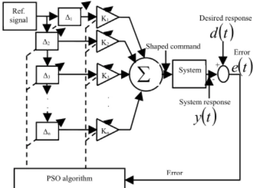
5.1. Command Shaping Using Gain and Delay Units 

A command shaping method is proposed using gain and 

diagram of the command shaping method is shown in Fig. 5. The 

unshaped reference signal is passed through multiple delay 

units,i, and then multiplied with gain factors, Ki. The shaped 

command is formed by summing up the delayed and weighted 

components. The effectiveness of the proposed method depends 

on a suitable selection of number of delay and gain elements and 

their corresponding values. For reasons of simplicity, the number 

of delay units and gain elements are kept the same. Assume that 

the number of gain elements and delay units are each represented 

by 

n

. In order to achieve the same level in the system’s response 

with the shaped command as with the unshaped reference, the 

gain values are selected in such a way that their sum is equal to 

unity [28, 34], i.e. 



  n i i K 1 1  (16) 

In order to minimise the delay in system’s response, the first 

delay unit is set to zero, i.e.,10. The values of the remaining 

delay units, 2,3,...n and all gain values, K1,K2,...,Kn may 

be derived analytically, as in a conventional command shaper [28, 

34]. 

 

Fig. 5. PSO‐based command shaping scheme using gain and 

delay elements 

Assuming that, no a priori information is available about the 

natural frequencies and associated damping ratios of the system, 

the proposed PSO algorithms are used to optimise the values of 

the gain and delay units so as to reduce vibration of the system. 

The error signal is calculated as: e

     

t d t yt ; where d

 

t , 

is the desired response and y

 

t  is the system actual response. 

An objective function is  formed using the error signal, as: 

 

x f

 

e

 

t

f  . This section presents two design examples, one 

with the proposed PSO and one with the MOPSO to demonstrate 

their effectiveness in designing controllers for flexible systems. 

5.2. Design Example‐1: Design of Command Shaping using PSO 

The  control  strategy  was  implemented  in  Simulink  [35] 

environment as shown in Fig. 6. The PSO process was encoded in 

Matlab .m files [36]. An interface was created so that the gain and 

delay values were calculated with PSO and passed to the 

Simulink environment and, after completion of the simulation, 

the system response was recorded and again passed to the PSO 

for further computation, and the process was repeated based on 

the initial population and total generation of the optimisation 

process. For n3, the number of gain elements is 3 and number 

of delay units is effectively 2, since the first delay unit is set to zero. 

The three gain units are termed as Gain 1, Gain 2 and Gain 3 and 

the corresponding values are indicated as K1, K2 and K3. The 

two delay units, associated with Gain 2 and Gain 3, are indicated 

as Delay 1 and Delay 2, respectively. The value of 

n

 was selected 

intuitively to keep resemblance with the number of impulses in a 

zero vibration derivative (ZVD) [34] type command shaper. The 

transfer function, as indicated in equation (15), is used in the 

Simulink model to characterise the vertical movement of the 

TRMS. 

For an evolutionary based design procedure, the searching 

capability of the algorithm is directly affected by the objective 

function. Moreover the design objective can only be achieved 

upon  suitable  selection  of  the  objective  function  of  the 

optimisation process. In the optimisation process, mean squared 

error (MSE) was used as the objective function. The main aim of 

the optimisation process is to reduce vibration in the vertical plane 

while the TRMS is in operation. In this example, feedforward 

control strategy is chosen where command shaping can be 

considered as the only controller. In such a case, the desired 

response of the system, d

 

t , is set to zero in order to achieve 

zero vibration while the system is in operation. So the system 

response,  y

 

t , is in fact considered as the error signal, e

 

t , 

which in turn is used to formulate the objective function, MSE, in 

the PSO optimisation process. 

 

Fig. 6. Simulink model of command shaping using gain and 

delay units 

a)   Parameter Encoding:   The PSO algorithm begins with a 

population of real numbers, called swarm. Each row represents a 

solution set, called particle. A swarm of ten particles with five 

elements each, i.e., 10 × 5 is created randomly within the range of 

[0, +1]. The first three elements of each individual are normalised 

and assigned to K1, K2 and K3.  In Matlab/Simulink [35, 36], 

the delay units are usually represented in terms of number of 

samples, which is an integer value. Thus, the remaining two 

elements of each individual are converted into integer numbers 

with a conversion factor of 0.01 followed by rounding operation 

and then assigned to Delay 1 and Delay 2 as indicated above. In 

the proposed PSO algorithm, the acceleration coefficients c1 and  2

c  were initially set to 1.5 whereas the inertia coefficient,



, was 

gradually  decreased  from  1.4  to  0.1  with  generation.  The 

acceleration coefficients,  c1 and c2, of each element of each 

particle are adjusted after every 

GEN

rep generations based on the 

Error

 

t e System response

 

t y Shaped command + -· · Ref. signal Δ1 Δ2 Δ3 Δn Kn · ·



System K3 K2 K1

PSO algorithm Error

Desired response

 

t d

shared fitness values of the particles. The value of 

GEN

rep was 

set as 10 in this case. The process was run for a maximum 

generation of 200. The algorithm was run for a maximum 

number of 200 generations and the values of gain and delay units 

of Simulink model (see Fig. 6) thus obtained with different values 

of 



s are presented in Table 1. Note that delay is calculated in 

terms of number of samples. 

Table 1. Values of gain and delay units* _{with different niche radii} 

for PSO  Niche radius  (s)  1 K   K2  K3  1  2  3  0.1  0.378  0.372  0.249  0  90  190  0.5  0.264  0.472  0.263  0  80  160  0.9  0.287  0.347  0.364  0  100  190 

Time‐domain performance measures of system response with 

shaped commands derived with different niche radii are shown 

in Table 2. The output response varies with the niche radius. The 

output response due to shaped command obtained at 



s 0.5 

produced better results compared to that with other values in 

terms of overshoot and settling time although there was a little 

increase in rise time. Among all these, the output response due to 

shaped command obtained with 



s= 0.5 seemed to be better as 

far  as overall performance  measures  were  concerned;  zero 

overshoot with satisfactory rise time, settling time and steady‐

state error. 

Table 2. Performance measures of output response due to shaped 

commands designed with different niche radii 

Niche  radius  (s)  Overshoot  (%)  Rise  time  (sec)  Settling  time  (sec)  Steady‐ state  error  0.1  4.445  1.5  18.7  0  0.5  1.53  1.6  2.0  0  0.9  3.489  1.5  13.6  0 

The convergence of the algorithm is shown in Fig. 7. The 

objective function of the best solution seems to either decrease or 

remain unchanged with generation due to the elitist property of 

the algorithm. 

 

Fig. 7. Convergence of the proposed variant of PSO 

The ‘mean objective function’ of the population decreases as 

the  algorithm  proceeds,  although  small  peaks  appear  that 

decrease with increasing generations. The occurrence of these 

peaks is attributed to the change in acceleration coefficients as 

discussed earlier. This change in acceleration coefficients after 

every 10 generations adds more diversity in the population which 

may extend the searching space in the optimisation process. The 

extra diversity in the swarm due to changes in c1 and c2 may 

lead to better solution. 

b)  Results:  The proposed variant of PSO was used to find the 

optimum values of gain and delay units. The algorithm was run 

for  200  generations  and  the  gain  values  obtained  are:   264

. 0 1

K , K20.472,  K30.263 and delay units are:  80

2

  and 3 160 (1 is set to zero). Here the delay units 

are represented in terms of number of samples. These values 

were obtained using MSE as objective function with 



s0.5. 

When the reference signal (bang‐bang) is passed through the gain 

and delay units and then added by a summation unit, the shaped 

signal is formed. Both the bang‐bang input and its corresponding 

shaped signal due to the above gain and delay values are shown 

in Fig. 8. For clarity, the leading edge is enlarged in Fig. 8, which 

also resembles a ZVD‐based shaped signal.    

 

Fig. 8. Bang‐bang input and shaped command input (time‐

domain)   

The time‐domain responses of the vertical channel due to 

bang‐bang input and shaped input are shown in Fig. 9. In order to 

highlight the differences in rise times, the leading edges of time‐

domain responses of the vertical channel due to bang‐bang input 

and shaped input are enlarged and shown in Fig. 10. It is noted 

that, speed of response of the vertical channel due to shaped 

command is slower compared to that due to bang‐bang input. It 

is  observed  that  oscillation  of  the  system  was  completely 

eliminated with shaped command and the system settled quickly 

to the steady‐state. Thus, the shaped command could improve 

several time domain performance measures, such as, overshoot 

and settling time with a slight decrease in system’s response. The 

frequency‐domain representation of the bang‐bang input and the 

shaped command are shown in Fig. 11 and the corresponding 

system responses are shown in Fig. 12. As noted, several troughs 

occur  in  the  frequency‐domain  representation  indicating  a 

decrease in energy level at those frequencies. Most importantly, 

the first trough occurs exactly at 0.7 Hz, where the main resonance 

at dominant mode to a large extent which in turn reduces the 

system vibration significantly (see Fig. 12). At the dominant mode 

(0.7 Hz) of the system, approximately 20dB attenuation was 

recorded with shaped command as the input relative to the 

response due to bang‐bang input.   

 

Fig. 9. Response of vertical channel due to bang‐bang signal and 

shaped command 

 

Fig. 10. Leading edges of time domain responses due to bang‐

bang signal and shaped command 

 

Fig. 11. Bang‐bang input and shaped command input (frequency‐

domain) 

5.3.  Design  Example‐2:  Design  of  Command  Shaping  using 

MOPSO 

For the TRMS, the command shaping technique, as designed 

with a single‐objective PSO causes a long delay in system’s 

response while it reduces vibration (see Fig. 10.).   For a flexible 

structure system, design objectives such as, the speed of system’s 

response and amount of vibration reduction are usually in conflict 

due to its construction and mode of operation. In practical design 

problems, a certain allowable range is specified for each objective 

and theoretical design method or a single‐objective optimisation 

process can hardly provide a solution satisfying both conflicting 

objectives  simultaneously.  The  single‐objective  based  design 

method can hardly provide good solutions where several (often 

conflicting) design objectives are to be met. In this section, taking 

the amount of vibration reduction and rise time as two competing 

objectives, the proposed MOPSO is used to design gain‐delay 

units based command shaper for the TRMS. 

 

Fig. 12. Response of vertical channel due to bang‐bang signal and 

shaped command 

a)  Implementation and MOPSO Solutions:  Root mean squared of 

error (RMSE) can be taken as a quantitative measure of overall 

vibration of the system in the time domain. Rise time of the 

system and RMSE are chosen as two objectives in the MOPSO 

process. The solution of MOPSO is not a single point, rather a set 

of solutions that trade off between these two conflicting objectives. 

For open loop response with a bang‐bang input signal, the rise‐

time and RMSE were recorded as 0.3 sec and 0.3241 respectively. 

The goal values of the design were chosen as less than or equal to 

0.3 for RMSE (objvective‐1) and less than or equal to 1.0 sec for 

rise‐time (objective‐2). The two objectives and the corresponding 

goal values are shown in Table 3. 

Table 3. Two objectives and goal values 

Objective  Parameter  Goal value 

Objective‐1  RMSE  ≤ 0.3 

Objective‐2  Rise‐time  ≤ 1 sec 

The control strategy was implemented in the Simulink [35] 

environment as shown in Fig. 6 and the MOPSO process was 

encoded in Matlab .m files [36]. The MOPSO algorithm begins 

with a population of real numbers called swarm. Each row 

represents a solution set called particle. A swarm of 20 particles 

with five elements each, i.e., 20 × 5 is created randomly within the 

range [0, +1]. The first  3 elements of each  individual  are 

normalized and assigned to gain elements, to K1, K2 and K3 

Matlab/Simulink, the delay units are usually represented in terms 

of number of samples which are integer numbers. Thus, the 

remaining 2 elements of the each individual are converted into 

integer numbers by a conversion factor of 0.01 using a ‘round’ 

operation and then assigned to  2 and  3 of the Simulink 

model. 

The acceleration coefficients were set as,c1c21.5, and 

inertia coefficient,



, was gradually decreased from 1.4 to 0.1 

with generation. The process was run for a maximum generation 

of 500. The maximum number of solutions that the external 

archive can keep is limited to 50. In order to maintain diversity 

among the solutions in the external archive, an adaptive grid 

mechanism was employed. For a two‐objective optimisation 

problem, the objective domain was divided into 49 (7×7) regions, 

called hyperparallelpids, as  shown in Fig. 3. The MOPSO 

algorithm with a population size of 20 individuals was run 

separately on this problem 6 times, each time for 500 generations. 

The number of non‐dominated solutions thus obtained with the 

algorithm at different runs is shown in Fig. 13.    0 2 4 6 8 10 12 14

run-1 run2 run-3 run-4 run-5 run-6

N o . of nondom in at ed s o lu ti ons  

Fig. 13. Numbers of non‐dominated solutions for proposed 

MOPSO algorithm at different runs 

Out of a total of 10000 points evaluated in each run, an average 

of only 10 were found to be non‐dominated relative to each other. 

In order to assess the performance of the MOPSO algorithm in 

this problem, the Pareto optimal set, obtained at run‐6, as shown 

in Fig. 14 is considered. In this plot, objective‐1 is represented on 

the horizontal axis and objective‐2 on the vertical axis. The 

number of non‐dominated solutions is 11 and 9 out of 11 

solutions remain within the range allowable for both objectives.   

 

Fig. 14. Pareto optimal set for MOPSO at run‐6 

b)  Results:  To validate the design approach as well as solution 

sets, one example solution is selected on the Pareto front as shown 

in Fig. 14. The example solution‐1 was chosen in such a way that 

the solution could yield satisfactory performance along both 

objective domains. If any particular objective is given priority in 

decision making, the designer can pick a solution from the non‐

dominated solution sets that satisfies the desired goal value along 

that objective domain. Two objective values for this solution are 

recorded as; RMSE = 0.3 and rise‐time = 0.4 sec. Here the RMSE is 

lower than that of open loop response with bang‐bang input 

whereas the rise‐time is slightly higher than that. Unshaped bang‐

bang input and shaped signal based on this example solution are 

shown in Fig. 15, where for clarity, the leading edge has been 

enlarged. The response of the vertical channel for unshaped bang‐

bang and shaped signal based on the example solution is 

presented in Fig. 16. A large oscillation is observed in the system 

response in the vertical channel with bang‐bang signal used as the 

input and the system takes long time to settle to a steady position. 

It is observed that oscillation of the system is significantly reduced 

with shaped command and the system settles quickly to the 

steady‐state. Thus, the shaped command could improve several 

time‐domain performance measures, such as, overshoot and 

settling‐time with a slight decrease in system’s response.   

 

Fig. 15. Bang‐bang input and shaped command input (time‐

domain) 

 

Fig. 16.  Response of vertical channel due to bang‐bang signal and 

shaped command 

Although the reduction of oscillation in system’s response is 

directly related to the reduction of vibration, frequency‐domain 

modes of the system and corresponding reduction at those 

modes. The frequency‐domain representation of the bang‐bang 

input and the shaped command is shown in Fig. 17 and the 

corresponding system response is shown in Fig. 18. 

It is observed from the system’s response due to bang‐bang 

signal that the system has only one dominant mode (peak in the 

frequency‐domain representation) which appears at 0.7 Hz. For 

bang‐bang input, the total energy seems to be evenly distributed 

throughout the band although it is higher near the DC level. On 

the contrary, several troughs occur in the frequency domain 

representation of