CEFAGE-UE Working Paper
2011/29
Pricing Longevity Bonds Using Affine-Jump Diffusion Models
Jorge Miguel Bravo
Pricing Longevity Bonds Using Affine-Jump Diffusion
Models
Jorge Miguel Bravo∗
Version: September 2011
Abstract
Historically, actuaries have been calculating premiums and mathematical reserves us-ing a deterministic approach, by considerus-ing a deterministic mortality intensity, which is a function of the age only, extracted from available (static) life tables and by setting a flat ("best estimate") interest rate to discount cash flows over time. Since neither the mor-tality intensity nor interest rates are actually deterministic, life insurance companies and pension funds are exposed to both financial and mortality (systematic and unsystematic) risks when pricing and reserving for any kind of long-term living benefits, particularly on annuities and pensions. In this paper, we assume that an appropriate description of the demographic risks requires the use of stochastic models. In particular, we assume that the random evolution of the stochastic force of mortality of an individual can be mod-elled by using doubly stochastic processes. The model is then embedded into the well known affine-jump framework, widely used in the term structure literature, in order to derive closed-form solutions for the survival probability. We show that stochastic mortal-ity models provide an adequate framework for the development of longevmortal-ity risk hedging tools, namely mortality-linked contracts such as longevity bonds or mortality derivatives.
JEL Code: G22
Keywords: stochastic mortality intensity; longevity risk; affine models; projected lifetables.
∗University of Évora - Department of Economics and CEFAGE-UE, Largo dos Colegiais, N.o
2, 7000-803, Évora/Portugal, Tel.: +351 266 740894, E-Mail: [email protected]. Paper presented at the Sixth Workshop on the "Consequences of longevity risks on pension systems and labor markets", Université Paris-Dauphine, Paris 3th-4th April 2008
1
Introduction
Longevity risk, i.e., the risk that members of some reference population might live longer, on average, than anticipated, has recently emerged as one of the largest sources of risk faced by life insurance companies, pension funds, annuity providers, life settlement investors and a number of other potential players in the marketplace for this risk. For example, given the uncertainty about future developments in mortality and life expectancy, pension funds and annuity providers run the risk that the net present value of their pension promises and annuity payments will turn out higher than expected, as they will have to pay out a periodic sum of income that will last for an uncertain life span.
This risk is amplified by the current problems in state-run social security systems. Given the long-term demographic trends observed in most developed countries (with low fertility rates and an ageing population), salaries and wages earned by active workers will have to finance the pensions of a growing number of retiree, making traditional pay-as-you-go social security systems unsustain-able. This will most likely force public pensions systems to moderate benefit promises in the future, reducing state-provided pension income. Additionally, the market trend away from defined-benefit corporate pension schemes towards defined-contribution plans and the move towards funded pension systems means that “Second Pillar” employer-related pension benefits will inevitably become more uncertain too. Moreover, traditional family networks in which the younger members of a family were encouraged to take care of the older ones, are being broken down by the extended mobility of the workforce.
In a scenario of unknown longevity, retirees can reduce the risk of exhausting assets before passing away by consuming less per year, but such a tactic then increases the chance that they might die with too much wealth left unconsumed. In other words, dying with too little wealth is undesirable, but having too much wealth is also undesirable, since it represents foregone consumption opportunities. In this scenario, individuals will have to become more self-reliant and will wish to diversify their sources of income in retirement, assigning in particular a greater weight to private solutions, namely annuities. As a consequence, annuity providers will face an increasing longevity risk.
These trends in mortality lead to the use of projected survival models when pricing and reserving for life annuities and other long-term living benefits. A number of different projection models have been proposed and are actually used in actuarial practice. In spite of this, the future mortality trend is actually random
and hence, whatever kind of model is adopted, systematic deviations from the forecasted mortality may take place.
The risk of systematic deviations is different in nature from that of random fluctuations around the trend, a well-known type of risk in the insurance business, in both the life and the non-life insurance areas. Effectively, the risk of systematic deviations arises from either a “model” or a “parameter” risk, which are unques-tionably non-pooling risks. Long-term trends observed in mortality affect both young and old ages. Although the terms “longevity risk” and “mortality risk” are very often used indistinctly, by longevity risk we mean the risk that members of some reference population might live longer, on average, than anticipated.
Longevity risk is a critical problem both because of the uncertainty of longevity projections, on one hand, and because of the huge amounts of liabilities at risk, on the other. Life annuities are probably the most important insurance product concerned by the longevity risk, but this risk should also be carefully considered when dealing with other long-term living benefits, insurance covers (particularly within the area of health insurance) and other retail products such as reverse mortgages. Additionally, many life insurers and reinsurers globally have become nervous about their exposure to catastrophic mortality events. This has resulted in the issuance of several bonds transferring mortality catastrophe risk to in-vestors.
Despite its significance, traditionally life companies and pension sponsors were short of solutions to manage longevity risk. Until recently, hedging strategies were limited to product redesign (e.g., participating annuities), to the adoption of conservative pricing policies, to the actuarial management of an insurer’s surplus (internal capital) and, in some cases, to the use of prospective lifetables.
In order for a market for hedging of longevity risk to develop there are several prerequisites. These include the development of generally accepted technology and models to quantify the risk and the successful design and implementation of financial products and markets to hedge the risk. There has been a significant increase in research addressing these issues in recent years, namely those involv-ing the securitization of risks, new capital market solutions and new reinsurance treaties.
In this paper, we assume that an appropriate description of the demographic risks requires the use of stochastic models. In particular, we assume that the random evolution of the stochastic force of mortality of an individual can be modelled by using doubly stochastic processes. The model is then embedded into the well know affine-jump framework, widely used in the term structure literature,
in order to derive closed-form solutions for the survival probability. We show that stochastic mortality models provide an adequate framework for the development of longevity risk hedging tools, namely mortality-linked contracts such as longevity bonds or mortality derivatives. The paper is organized as follows. In Section 2 we briefly review both the traditional “dynamic approach” and the new “stochastic mortality approach”. In Section 3 we use doubly stochastic processes in order to model the random evolution of the stochastic force of mortality in a manner that is common in the credit risk literature. The model is then embedded into the well know affine-jump term structure framework, widely used in the term structure or credit risk literature, in order to derive closed-form solutions for the survival probability. In Section 4 we calibrate the model to the Portuguese projected lifetables. Results indicate that the model is flexible enough to accommodate the rectangularization phenomena and that jumps seem to be an appropriate way to describe the random variations observed in mortality. Section 5 concludes.
2
Modeling mortality and longevity risk
One of the key conditions for the development of longevity-linked products and markets and for the hedging of longevity risk is the development of generally agreed market models for risk measurement. Whereas traditional market risks such as equity market, interest rate, exchange rate, credit and commodity risks have well consolidated methodologies for quantifying risk-based capital and for establishing market prices, longevity and mortality risk has historically been a very opaque risk. For a long time, only demographers, actuaries and insurance companies showed any interest in measuring and managing this risk, mainly for pricing purposes. A number of explanations can be given for this, particularly the fact that it is a non-financial risk that has been measured and analyzed in a different way from financial risks, generally adopting deterministic or scenario based approaches.
Historically, actuaries have been calculating premiums and mathematical re-serves using a deterministic approach, by considering a deterministic mortality intensity, which is a function of the age only, extracted from available (static) lifetables and by setting a flat (“best estimate”) interest rate to discount cash flows over time. Since neither the mortality intensity nor interest rates are ac-tually deterministic, life insurance companies are exposed to both financial and mortality (systematic and unsystematic) risks when pricing and reserving for any kind of long-term living benefits, particularly on annuities. In particular, the
cal-culation of expected present values requires an appropriate mortality projection in order to avoid significant underestimation of future costs.
In order to protect the company from mortality improvements, actuaries have different solutions, among them to resort to projected (dynamic or prospective) lifetables, i.e., lifetables including a forecast of future trends of mortality instead of static lifetables. Static lifetables are obtained using data collected during a specific period (1 to 4 years) whereas dynamic lifetables incorporate mortality projections. To illustrate the problems with this approach, consider a female individual born in 2006. Her mother is 30-year-old and her grand-mother 60. To estimate the life expectancy of the newborn, the death probability at age 30 will be her mother’s one and at age 60 her grand-mother’s one, observed in 2006. This means that in a situation where longevity is increasing, static lifetables underestimate lifelengths and thus premiums relating to life insurance contracts. Conversely, dynamic lifetables will project mortality into the future accounting for longevity improvements.
Since the future mortality is actually unknown, there is enormous likelihood that future death rates will turn out to be different from the projected ones, and so a better assessment of longevity risk would be one that consists of both a mean estimate and a measure of uncertainty. Such assessment can only be performed using stochastic models to describe both demographic and financial risks. In this section, we briefly review both the traditional “dynamic approach” and the new “stochastic mortality approach”.
2.1 Discrete-time dynamic approach
Although the subject of estimating future levels of mortality has received enor-mous attention lately, actuarial models of mortality and life tables for pricing and projecting pension and related life product cash flows have been developed over centuries. Tuljapurkar and Boe (1998), Tabeau (2001), GAD (2001), Pitacco (2004), Wong-Fupuy and Haberman (2004), Booth (2006) and Bravo (2007) pro-vide a detailed review of historical patterns in mortality and longevity forecasting models.
In such a sensitive issue, there are a number of different opinions regarding how long people will live in the future. Some argue that lifespans will continue to increase at least as rapidly as experienced over the last decades due to, e.g., new medical breakthroughs or healthier life styles. Others disagree and project that increases in lifetime will decelerate, and potentially even decline (at least for certain risk groups), since any increase in longevity would have to occur by virtue
of declines in mortality for older age groups, or for other underlying causes of death. Other controversial points in this debate refer to the possible existence of a biological limit to human life and whether we are actually approaching it (see, e.g., Vaupel (1997), Olshansky and Carnes (1997) and Watson Wyatt (2005)).
The competing views on the evolution of lifespans, medical advancement or the existence of a biologic limit to human life translate into the question of how to appropriately model future longevity. Mortality forecasting methods currently in use can be categorized in many different ways. They can be clustered into epi-demiological methods, projection by cause of death, extrapolative models, expert-opinion models and relational models.
Epidemiological models analyze the relationship between specific risk factors (e.g., smoking, obesity, socio-economic status, marital status and specific diseases) and their effects on mortality. The idea is to estimate the impact of specified risk factors on mortality rates (not on causes of death), from which mortality forecasts can be generated by projecting these risk factors into the future, given certain distributional assumptions. The practical usefulness of this approach lacks an accurate knowledge of the relationship between risk factors and mortality, something that science may achieve in the future. In relational models, future mortality rates are assumed to follow the dynamics of observed mortality for a more “advanced” population. The assumption is that the mortality profile of the forecasted population (e.g., of a developing country) will converge to the “target” population over some future time horizon.
Extrapolative models assume that future mortality can be estimated by pro-jecting into the future the same trends observed in the recent to medium-term past. While the models can be either deterministic or stochastic, the basic idea is that future mortality will continue to improve at the same rate as in the past (observation window). This approach is the most popular among official bureaus all over the world but should be used with caution since it depends on the reli-ability of base mortality data and neglects, to a certain extent, the uncertainty related to the evolution of causes of death, future medical advances or to envi-ronmental risk factors. A variant of this approach are the methods that involve projection by cause of death, i.e., methods that disaggregate total mortality and forecast mortality rates for each cause of death separately by extrapolating past trends. Finally, expert-opinion models are also based on an extrapolative model, but explicitly include assumptions by the forecaster in respect to the future evolu-tion of mortality. The idea is to incorporate addievolu-tional informaevolu-tion not captured by the statistical model ensuring that forecasted values are not pushed beyond
reasonable limits.
The classical approach to incorporating improvement in longevity for forecast-ing future mortality within extrapolative models is to fit an appropriate paramet-ric function (e.g., Makeham model) to each calendar year data. Then, each of the parameter estimates is treated as independent time series, extrapolating their behaviour to the future in order to provide the actuary with projected lifetables (see, e.g., CMIB (1976) and Heligman e Pollard (1980)). Despite simple, this approach has serious limitations. In the first place, the approach strongly relies on the appropriateness of the parametric function adopted. Secondly, parameter estimates are very unstable, a feature that undermines the reliability of univariate extrapolations. Thirdly, the time series for parameter estimates are not indepen-dent and often robustly correlated. Although applying multivariate time series methods for the parameter estimates is theoretically possible, this will complicate the approach and introduce new problems.
Lee and Carter (1992) developed a simple model for describing the long term trends in mortality as a function of a simple time index. The method models the logarithm of a time series of age-specific death ratesµx(t) as the sum of an age-specific componentαx,that is independent of time, and a second component, expressed as a product of a time-varying parameter denoting the general level of mortalityκt, and an age-specific component βx that signals the sensitiveness of mortality rates at each age when the general level of mortality changes. Formally, we have
lnµx(t) =αx+βxκt+ǫx,t, (1) whereǫx,t ∼ Nor
0, σ2ǫis a white-noise, representing transitory shocks and the
parameters αx,βx and κthave to be constrained by tmax t=tmin κt= 0 and xmax x=xmin βx = 1, (2)
in order to ensure model identification.
Parameter estimates are obtained by ordinary least squares, i.e., by solving the following minimization program
(ˆαx,βˆx,ˆκt) = arg min αx,βx,κt xmax x=xmin tmax t=tmin (lnµx(t)−αx−βxκt)2 . (3)
Lee and Carter (1992) solve (3) by resorting toSingular Value Decomposition
consider-ing iterative methods (see, e.g., Bravo (2007)) or Weighted Least-Squares (see, e.g., Wilmoth (1993)). The resulting time-varying parameter estimates are then modeled and forecasted using standard Box-Jenkins time series methods. Finally, from this forecast of the general level of mortality, projected age-specific death rates are derived using the estimated age-specific parameters.
There have been several extensions to the Lee-Carter model including different error assumptions and estimation procedures. Lee (2000), Lee and Miller (2001), Tuljapurkar and Boe (1998), Brouhnset al. (2002a), Wong-Fupuy and Haberman
(2004), Bravo (2007) and Cairnset al. (2007) discuss the model and extensions.
Brouhnset al. (2002a) and Renshaw and Haberman (2003c) develop an extension
of the Lee-Carter model allowing for Poisson error assumptions and apply the model to Belgian data. This Poisson log-bilinear approach can be stated as
Dx,t ∼ Poisson(µx(t)Ex,t), (4) where Dx,t denotes the number of deaths recorded at age x during year t, from an exposure-to-risk (i.e., the number of person-years from whichDx,t arise),Ex,t, and µx(t) is given by (1).
One of the main advantages of the Poisson log-bilinear model over the Lee-Carter model is that specification (4) allows us to use maximum-likelihood ods to estimate the parameters instead of resorting to least squares (SVD) meth-ods. Formally, we estimate the parameters αx, βx and κt by maximizing the log-likelihood derived from model (1)-(4)
lnV(α,β,κ) = tmax t=tmin xmax x=xmin {Dx,t(αx+βxκt)−Ex,texp (αx+βxκt)}+c, (5)
where α = (αxmin, . . . , αxmax)′, β =
βxmin, . . . , βxmax′, κ = (κxmin, . . . , κxmax)′ and cis a constant.
The presence of the bilinear term βxκt makes it impossible to estimate the model using standard statistical packages that include Poisson regression. Be-cause of this, we resort to an iterative method for estimating log-linear models with bilinear terms proposed by Goodman (1979). Even with a Poisson error assumption, heterogeneity by age-group in mortality indicates over-dispersion of errors.
Empirical studies to date suggest the need for more than a single factor to model longevity improvement, something that the Lee-Carter approach with a single factor and varying improvement impacts by age does not appear to capture.
This is important because if pricing models can often perform reasonably well with only a single factor, hedging requires a more complete picture of the dynamics of longevity improvements. In this sense, Bell (1997), Booth et al. (2002) and
Renshaw and Haberman (2003c,d) include a second log-bilinear term in (1) and estimate parameters by considering the first two term in a SVD. Additionally, they adopt a multivariate setting in order to project the evolution of the time indicesκt,i (i= 1,2,).
Carter and Prskawetz (2001) consider the possibility of time varying parame-ters αx and βx. Renshaw and Haberman (2003a) include additional non-linear age factors when modeling the so-called “mortality reduction factors” within a Generalized Linear Models (GLM’s) approach. Renshaw and Haberman (2006) and Currieet al. (2004) include a cohort factor including year of birth as a factor
impacting the rate of longevity improvement. This cohort factor is found to be significant in UK mortality data. Renshaw e Haberman (2005) and Bravo (2007) develop a version of the Lee-Carter model considering positive asymptotic mortal-ity. This result is, for most age groups, more consistent with observed mortality patterns when compared with that of the original model. Wilmoth and Valkonen (2002) develop an extension of the Lee-Carter model aimed to investigate differ-ential mortality by considering a number of alternative covariates other than age and calendar time.
Cairns, Blake and Dowd (2006b) develop and apply a two-factor model similar to the Lee-Carter model with a smoothing of age effects using a logit transfor-mation of mortality rates. Cairns et al. (2007) analyze England and Wales and
US mortality data showing that models that allow for an age effect, a quadratic age effect and a cohort effect fit the data best although the analysis of error dis-tributions in these models revealed disappointing. De Jong and Tickle (2006) formulate the Lee-Carter model in astate space framework.
2.2 Stochastic mortality modeling
Models following the approach of Lee and Carter typically adapt discrete-time time series models to capture the random element in the stochastic development of mortality rates. Given the unknown nature of future mortality, some authors have recently developed models in a continuous-time framework by modeling mortality intensity as a stochastic process (see, e.g., Milevsky and Promislow (2001), Dahl (2004), Biffis and Millossovich (2004, 2006), Biffis (2005), Dahl and Møller (2005), Miltersen and Persson (2005), Cairnset al. (2006a), Schrager (2006), Bravo (2007)
Modeling the mortality intensity as a stochastic process allows us to capture two of its more significant features: time dependency and uncertainty of the future development. Additionally, this framework provides a more accurate description of both premiums and liabilities of life insurance companies and contributes to a proper quantification of systematic mortality risk (also called longevity risk) faced by them. This framework and model application provides the theoretical foundation for financial pricing of longevity dependent financial claims and for the development of longevity risk hedging tools, namely mortality-linked contracts such as longevity bonds or other longevity-linked derivatives.
Up to now, a number of different stochastic mortality models have been pro-posed - for a detailed classification see Cairns et al. (2006a) and Bravo (2007).
Most of these stochastic mortality models are short rate mortality models, i.e.,
they model the spot mortality rate qx(t), or the spot force of mortality µx(t). We can also find forward mortality models, i.e., approaches that model the
dy-namic of the forward mortality intensity fxµ(t, T), a positive-mortality modeling
framework for the spot survival probability px(t),in line with the term structure approach developed by Flesaker e Hughson (1996), Rogers (1997) and Rutkowski (1997), or market-models for the forward survival probability.
Milevsky and Promislow (2001) were the first to propose a stochastic “hazard rate” or force of mortality. With the intention of pricing guaranteed annuitiza-tion opannuitiza-tions in variable annuities, the authors demonstrate, first in a discrete-time framework, how to price and hedge a plain vanilla mortality option using a portfo-lio composed by zero coupon bonds, insurance contracts and endowment contracts. Moreover, they price the same option in a continuous-time risk-neutral framework assuming that the dynamics of the short interest rate and of the mortality inten-sity evolve independently over time according to a Cox-Ingersoll-Ross-process and a stochasticmean reverting Brownian Gompertz-type model, respectively.
Dahl (2004) develops a general stochastic model for the mortality intensity. The author derives partial differential equations for both the price at which some insurance contracts should be sold on the financial market and for the general mor-tality derivatives in the presence of stochastic mormor-tality. In addition, he envisages solutions by which systematic mortality risk can be transferred to the financial market. Dahl and Moller (2005) derive risk-minimizing strategies for insurance liabilities in a market without derivative securities. Biffis and Millossovich (2004) expand this framework to a bidimensional setting in order to deal effectively with several sources of risk that simultaneously affect insurance contracts.
finan-cial and demographic factors. Specifications of the model with an affine term structure are employed and closed form mathematical expressions (up to the so-lutions of standard Riccati ordinary differential equations) are derived for some classic life insurance contracts. In Section?? we illustrate this approach with a particular example.
Schrager (2006) presents an affine stochastic mortality model, that simulta-neously describe the evolution of mortality for different age groups as opposed to the previous formulation in which a single cohort is considered. The author fits the model to Dutch mortality data using Kalman filters and presents alternative valuation approaches for a number of mortality-contingent contracts.
Biffis and Denuit (2005) and Biffis et al. (2006) generalize the model
pro-posed by Lee and Carter (1992) to a stochastic setting. The authors assume that the dynamics of the time-varying parameter κt can be described by stochastic differential equations.
While most of the models presented so far assume independence between fi-nancial and demographic risk factors, Miltersen and Persson (2005) allow for cor-relations. The authors adopt the well know Heath-Jarrow-Morton no-arbitrage approach and model the forward mortality intensity (instead of the spot mortal-ity intensmortal-ity), taking the whole forward-mortalmortal-ity curve as an infinite-dimensional state variable. Similar to standard term structure literature, they derive no-arbitrage conditions for the drift term.
These models have generally been implemented for single age cohorts. To al-low for multiple ages in the modeling, dependence across ages must be modeled in a proper way. Although these arbitrage-free models currently provide the most potential as a standard modeling framework for pricing and hedging longevity risk based products, there are a number of modeling issues that need to be addressed and that are yet to be fully explored. Important issues include the modeling of morbidity and ill-health, the use of multiple state models to capture the de-pendence between competing risk factors or incorporating cause of death as risk factors.
3
Affine-Jump diffusion processes for mortality
In this section we draw a parallel between insurance contracts and certain credit-sensitive securities and exploit some results of the intensity-based approach to credit risk modeling. Specifically, we use doubly stochastic processes (also known asCox processes) in order to model the random evolution of the stochastic force
of mortality of an individual aged x in a manner that is common in the credit
risk literature. The model is then embedded into the well know affine-jump term structure framework, widely used in the term structure literature, in order to derive closed-form solutions for the survival probability.
3.1 Mathematical framework
We are given a filtered probability space (Ω,F,F,P) and concentrate on an
indi-vidual aged x at time0.Following the pioneering work of Artzner and Delbaen
(1995) in the credit risk literature and the proposals by Dahl (2004) and Biffis (2005) among others in the mortality area, we model his/her random lifetime as anF-stopping timeτx admitting a random intensityµx.Specifically, we consider
τx as the first jump-time of a nonexplosive F-counting process N recording at each time t ≥0 whether the individual has died (Nt= 0) or survived (Nt= 0). The stopping time τx is said to admit an intensityµx if the compensator of N does, i.e., ifµx is a nonnegative predictable process such that0tµx(s)ds <∞for
allt≥0 and such that the compensated processMt=
Nt−0tµx(s)ds:t≥0
is a localF-martingale. If the stronger condition E t
0µx(s)ds
<∞is satisfied,
thenMt is anF-martingale. From this, we derive
E(Nt+∆t−Nt| Ft) =E t+∆t t µx(s)ds Ft , (6)
based on which we can write
E(Nt+∆t−Nt| Ft) =µx(t)∆t+o(∆t), (7) an expression comparable with that of the instantaneous probability of death
∆tqx+t derived in the traditional deterministic context.
By further assuming thatN is a Cox (or doubly stochastic) process driven by
a subfiltration G of F,with F-predictable intensity µ it can be shown, by using
the law of iterated expectations, that the probability of an individual agedx+t
at timetsurviving up to timeT ≥t,on the set{τ > t},is given by
P(τ > T| Ft) =Ee− T t µx+s(s)ds Ft . (8)
Readers who are familiar with mathematical finance and, in particular, with the interest rate literature, can without difficulty observe that the right-hand-side of equation (8) represents the price at timetof a unitary default-free zero coupon
bond with maturity at timeT > t,if the intensityµis to represent the short-term
interest rate.
One of the main advantages of this mathematical framework is that we can approach the survival probability (8) by using well known affine-jump diffusion processes. In particular, an Rn-valued affine-jump diffusion process X is an F
-Markov process whose dynamics is given by
dXt=δ(t, Xt)dt+σ(t, Xt)dWt+ m h=1
dJth, (9)
where W is a F-standard Brownian motion in Rn and each component Jh is
a pure-jump process in Rn with jump-arrival intensity ηh(t, X
t) :t≥0 and time-dependent jump distributionνht on Rn. An important requirement of affine
processes is that the drift δ : D → Rn, the instantaneous covariance matrix
σσT :D →Rn×n and the jump-arrival intensity ηh :D →R
+ must all have an
affine dependency onX . The jump-size distribution is determined by its Laplace
transform.
The convenience of adopting affine processes in modeling the mortality inten-sity comes from the fact that, for anya∈Cn,for givenT ≥tand an affine function
Rdefined by R(t, X) =ρ0(t) +ρ1(t)·X,under certain technical conditions we
have φX(a, Xt, t, T)⊜E e− T t R(s,Xs)dsea·XT Ft =eα(t)+β(t)·Xt, (10)
where α(·) =. α(·;a, T), β(·) =. β(·;a, T) satisfy generalized Ricatti ordinary
differential equations, that can be solved at least numerically and, in some cases, as we will see below, analytically.
3.2 Mortality intensity as a stochastic process
Turning now to the problem of modeling adequately the dynamics of mortality, we illustrate the approach developed in the previous section by developing a new model for the mortality intensity that considers the classic Feller equation together with a jump component. Formally, we assume that the mortality intensityµx+t(t)
solves the following stochastic differential equation
dµx+t(t) =aµx+t(t)dt+σµx+t(t)dW(t) +dJ(t) (11)
with J(t) = Nt i=1 εi. (12)
whereµ¯x>0, a >0,σ ≥0 and W(t)is a standard Brownian motion.
We assume thatJ(t) is a compound Poisson process, independent ofW, with
constant jump-arrival intensity η ≥ 0, where {εi:i= 1, . . . ,∞} are i.i.d. vari-ables. Following the results by Kou (2002), among others, we consider jump sizes that are random variables double asymmetric exponentially distributed with density f(z) =π1 1 υ1 e− z υ1I {z≥0}+π2 1 υ2 e z υ2I {z<0} (13) where π1, π2 ≥ 0, π1 +π2 = 1, represent, respectively, the probabilities of a
positive (with average sizeυ1>0) and negative (with average sizeυ2>0) jump.
By settingπ1 = 0we are interested only on the importance of longevity risk (see,
e.g., Biffis (2005)). By setting η = 0 the model becomes deterministic. When
υ1 =υ2 and π1 =π2 = 12 we get the so-called “first Laplace law”. By adopting
equation (13) we consider the significance of both positive mortality shocks (e.g., new medical breakthroughs) and negative mortality shifts (e.g., bird flu).
In the spirit of (10), let us now assume that the survival probabilityT−tpx+t(t) is represented by an exponentially affine function. By applying the framework described above, we have that
T−tpx+t(t)≡eA(τ)+B(τ)·µx+t(t) (14) whereτ =T−t.
It can be shown that the solution to this problem admits the following Feynman-Kac representation υt, µx+t(t) −A˙(τ)−B˙(τ)µx(t) +aµx+t(t)B(τ) +σ 2 2 µx+t(t)B 2(τ) +η π1 1−υ1B(τ) + π2 1 +υ2B(τ) −1 −µx+t(t) = 0, (15) whereυt, µx+t(t)=T−tpx+t(t).
Dividing both sides of this equation by υt, µx+t(t)we get
−B˙(τ) +aB(τ) +σ 2 2 B 2(τ)−1µ x+t(t) (16) + −A˙(τ) +η π1 1−υ1B(τ) + π2 1 +υ2B(τ)−1 = 0,
whereA(τ) andB(τ) are solutions to the following system of ODEs’ ˙ B(τ) = aB(τ) +1 2σ 2B2(τ)−1 (17) ˙ A(τ) = η π 1 1−υ1B(τ) + π2 1 +υ2B(τ) −1 (18) with boundary conditions
B(0) = 0, A(0) = 0. (19)
whereB˙(τ) = ∂τ∂ B(τ),A˙(τ) = ∂τ∂ A(τ).
By solving the system (17)-(18)-(19), we get the following closed-form solutions forA(τ) and B(τ) A(τ) = ηπ1 α 0τ (α0−υ1) + υ1(α0+α1) [ln (α0+α1)−ln (α0−υ1+ (α1+υ1)eκτ)] κ(α0−υ1) (α1+υ1) +ηπ2 α 0τ (α0+υ2) + υ2(α0+α1) κ(α1−υ2) (α0+υ2)[−ln (α0+α1) (20) + ln (α0+υ2+ (α1−υ2)eκτ)]} −ητ B(τ) = 1−e κτ α0+α1eκτ (21) withκ=√a2+ 2σ2, α
0 = (a+2κ) and α1 = (κ−2a), defined for
−υ1
2
<B(τ)< 1
υ1. (22)
We observe that the model stipulates an increasing (deterministic) trend for the mortality intensity, around which random fluctuations occur due to the sto-chastic component and due to the jump component. Additionally, the model offers a realistic process for the stochastic mortality rate since it ensures that the variable cannot take negative values. The model assumes that both negative and positive jumps can be registered in mortality, a feature that contrasts with similar models that are interested in sudden improvements in mortality (e.g., due to medical advances) only. We think this gives a more appropriate description of mortality, in which unexpected increases in mortality can occur (e.g., caused by natural catastrophes or epidemics). The model offers a nice analytical solution, easy to use in pricing and reserving applications within the life insurance industry.
4
Calibration to the Portuguese projected lifetables
As a first application of the above models, we have calibrated model (11) to the Portuguese projected lifetables. Portuguese projected lifetables were obtained by fitting model (4)-(1)-(2) to a matrix of crude Portuguese death rates, from year 1970 to 2004 and for ages0 to84.The data, discriminated by age and sex, refers
to the entire Portuguese population and has been supplied by the Portuguese National Institute of Statistics (INE - Instituto Nacional de Estatística). The database used comprised two elements: the observed number of deathdx,t given by age and year of death, and the observed population size lx,t at December 31 of each year. We follow the INE definition of population at risk using the
population counts at the beginning and at the end of a year and take migration into account. The Poisson parametersαx, βxandκtimplicated in (1) are estimated by maximum-likelihood methods using the iterative procedure described in Section 2.1.1
The closing of lifetables was performed using the method proposed by De-nuit and Goderniaux (2005) to extrapolate mortality rates at very old ages. The method is a two step method. First, a quadratic function is fitted to age-specific estimated mortality rates in a given age-band. Second, the estimated function is used to extrapolate mortality rates up to a pre-determined maximum age. For-mally, the following log-quadratic model is fitted by weighted least-squares
ln ˆqx(t) =a(t) +b(t)x+c(t)x2+ǫx(t), x∈[65,84] (23) to age-specific mortality rates observed at older ages (in our case x ∈ [65,84]), whereǫx(t)∼ N0, σ2(t), with additional constraints
qxmax = 1 (24)
qxmax′ = 0 (25)
whereq′x denotes the first derivative of qx with respect to age xmax. Constraints
(24) and (25) impose a concave configuration to the curve of mortality rates at old ages and the existence of a horizontal tangent at x = xmax = 120. We then
use this function to extrapolated mortality rates up to agexmax.
In fitting the model, we have adopted the ordinary least squares method, i.e., we minimize the quadratic deviations between the model survival probabilities, T−tpmodel65 (t),and the prospective lifetable ones, T−tpTP65 (t) for an individual aged
65. Formally, parameter estimatesΘsolve the following optimization problem ˆ Θ = arg min Θ Q 2 = t+(xmax−65)+1 T=t+1 T−tpmodel65 (t)−T−tpTP65(t) 2 (26)
wherexmax= 120 andt∈ {1970,1980,1990,2004}.
Table 1 reports the optimal values of the parameters, the calibration error and the initial value of µx+t(t), µ65(t), chosen to be equal to −ln (p65(t)), for
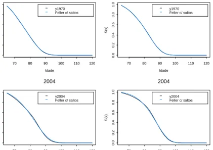
both male and female populations. Figure 1 report, for the generations aged 65
int∈[1970,2004],the survival function of the stochastic process analysed and of
the prospective lifetable one.
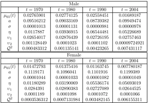
Male t= 1970 t= 1980 t= 1990 t= 2004 µ65(t) 0.02765901 0.02774125 0.02558451 0.01689187 a 0.09516212 0.09033169 0.08739382 0.09949474 σ 0.00001013 0.00001131 0.00000981 0.00000978 η 0.0117887 0.03936915 0.06544481 0.05226689 υ1 0.02654017 0.02876439 0.02726195 0.02757463 υ2 0.001128449 0.0001023 0.0001102 0.00009724921 Q2 0.000483312 0.001135141 0.00423265 0.007431117 Female t= 1970 t= 1980 t= 1990 t= 2004 µ65(t) 0.01472793 0.01375416 0.01163745 0.007780187 a 0.1119171 0.1096041 0.1101916 0.1199389 σ 0.00001044 0.00001033 0.00001082 0.00001049 η 0.01180289 0.03190069 0.05536174 0.05693019 υ1 0.0284391 0.02890383 0.02727089 0.02644525 υ2 0.0001189 0.0001098 0.0001072 0.0001066 Q2 0.0003536312 0.0007131984 0.003482145 0.006155311
Table 1: Parameter estimates
The calibration error is quite small and the parameter estimates show that the value ofσ is very low, particularly when compared with that of both positive
and negative average size jumps. We can observe that the fit is very good, even when we consider the importance of the rectangularization phenomena, highly significant in the 2004 generation. The results also suggest that jumps seem to be an appropriate way to describe the random variations observed in mortality.
1970 Idade S (x ) 70 80 90 100 110 120 0 .0 0 .2 0 .4 0 .6 0 .8 1 .0 y1970 Feller c/ saltos 1970 Idade S (x ) 70 80 90 100 110 120 0 .0 0 .2 0 .4 0 .6 0 .8 1 .0 y1970 Feller c/ saltos 2004 Idade S (x ) 70 80 90 100 110 120 0 .0 0 .2 0 .4 0 .6 0 .8 1 .0 y2004 Feller c/ saltos 2004 Idade S (x ) 70 80 90 100 110 120 0 .0 0 .2 0 .4 0 .6 0 .8 1 .0 y2004 Feller c/ saltos
Figure 1: Survival probabilityT−tp65(t)as a function of agex+T−tfort= 1970
and t= 2004 (the left panel corresponds to the male population)
5
Conclusion
In this paper, we have reviewed both the traditional discrete-time dynamic ap-proach to mortality projection and the new “stochastic mortality apap-proach” to mortality and longevity risk modeling. We have describe the random evolution of mortality by using doubly stochastic processes. The intensity is then described as an affine-jump diffusion process, considering jump sizes that are random variables double asymmetric exponentially distributed. The model is compatible with both both negative and positive jumps in mortality, a feature that contrasts with sim-ilar models that are interested in sudden improvements in mortality (e.g., due to medical advances) only. Survival probabilities have been provided in closed-form. The intensity process has been calibrated to the Portuguese population using pro-jected lifetables built using the Poisson Lee-Carter method. The results show that fit is very good and that the model is flexible enough to accommodate some of the traditional demographic phenomena.
References
[1]Artzner, P. and Delbaen, F. (1995). Default risk insurance and incomplete markets. Mathematical Finance, 5(3), 187-195.
[2]Ballotta, L. and Haberman, S. (2006). The fair valuation problem of guaran-teed annuity options: The stochastic mortality environment case. Insurance: Mathematics and Economics, 38, 195-214.
[3]Bell, W. (1997). Comparing and assessing time series methods for forecasting age specific demographic rates.Journal of Official Statistics, 13, 279-303.
[4]Biffis, E. (2005). Affine processes for dynamic mortality and actuarial valua-tions. Insurance: Mathematics and Economics, 37, 443-468.
[5]Biffis, E. and Denuit, M. (2005). Lee Carter Goes Risk-Neutral: An Applica-tion to the Italian Annuity Market. Actuarial Research Paper N.o 166, Fac-ulty of Actuarial Science and Statistics, Cass Business School, City University, London.
[6]Biffis, E. and Millossovich, P. (2004). A Bidimensional Approach to Mortality Risk. Working Paper, Università Bocconi
[7]Biffis, E. and Millossovich, P. (2006). The fair value of guaranteed annuity options.Scandinavian Actuarial Journal, 1, 23-41.
[8]Biffis, E., Denuit, M. and Devolder, P. (2006). Stochastic mortality under measure changes. Actuarial Research Paper, Faculty of Actuarial Science and
Statistics, Cass Business School, City University, London.
[9]Booth, H., Maindonald, J. and Smith, L. (2002). Applying Lee-Carter under conditions of variable mortality decline.Population Studies, 56, 325-336. [10]Bravo, J. M. (2007). Tábuas de Mortalidade Contemporâneas e Prospectivas:
Modelos Estocásticos, Aplicações Actuariais e Cobertura do Risco de Longev-idade. PhD Thesis, University of Évora, Portugal.
[11]Brouhns, N., Denuit, M. and Vermunt, J. (2002a). A Poisson log-bilinear re-gression approach to the construction of projected lifetables.Insurance: Math-ematics and Economics, 31, 373-393.
[12]Cairns, A., Blake, D. and Dowd, K. (2006a). Pricing Death: Frameworks for the Valuation and Securitization of Mortality Risk. ASTIN Bulletin, 36,
[13]Cairns, A., Blake, D. and Dowd, K. (2006b). A Two-Factor Model for Sto-chastic Mortality with Parameter Uncertainty: Theory and Calibration. The Journal of Risk and Insurance, 73(4), 687-718.
[14]Cairns, A., Blake, D., Dowd, K., Coughlan, G.D., Epstein, D., Ong, A., and Balevich, I. (2007). A quantitative comparison of stochastic mortality models using data from England and Wales and the United States. Cass Business School.
[15]Carter, L. and Prskawetz, A. (2001). Examining structural shifts in mortality using the Lee-Carter method. Max Planck Institute for DemographicResearch
WP 2001-007, Germany.
[16]CMIB (1976). Mortality Investigation Reports, CMIR 2. The Institute of
Ac-tuaries and Faculty of AcAc-tuaries, UK.
[17]Currie, I., Durban, M. and Eilers, P. (2004). Smoothing and forecasting mor-tality rates. Statistical modeling, 4, 279-298.
[18]Dahl, M. (2004). Stochastic Mortality in Life Insurance: Market Reserves and Mortality-Linked Insurance Contracts. Insurance: Mathematics and Eco-nomics, 35, 113-136.
[19]Dahl, M. and Moller, T. (2005). Valuation and hedging of life insurance liabil-ities with systematic mortality risk. In Proceedings of the 15th International AFIR Colloquium, Zurich.
[20]De Jong, P. and Tickle, L. (2006). Extending Lee-Carter mortality forecasting.
Mathematical Population Studies, 13(1), 1-18.
[21]Flesaker, B. and Hughson, L. (1996). Positive interest. Risk, 9(1), 46-49.
[22]GAD — Government Actuary’s Department (2001).National Population Pro-jections: Review of Methodology for Projecting Mortality. Report N.o 8,
Lon-don.
[23]Goodman, L. (1979). Simple models for the analysis of association in cross classifications having ordered categories. Journal of the American Statistical Association, 74, 537-552.
[24]Heligman, L. and Pollard, J. (1980). The age pattern of mortality.Journal of the Institute of Actuaries, 107, 49-80.
[25]Kou, S. (2002). A jump-diffusion model for option pricing. Management Sci-ence, 48, 1086-1101.
[26]Lee, R. (2000). The Lee-Carter method for forecasting mortality, with various extensions and applications.North American Actuarial Journal, 4(1), 80-93.
[27]Lee, R. and Carter, L. (1992). modeling and forecasting the time series of US mortality.Journal of the American Statistical Association, 87, 659-671.
[28]Lee, R. and Miller, T. (2001). Evaluating the performance of the Lee-Carter approach to modeling and forecasting. Demography, 38, 537-549.
[29]Milevsky, M. and Promislow, S. (2001). Mortality derivatives and the option to annuitise.Insurance: Mathematics and Economics, 29, 299-318.
[30]Miltersen, K. and Persson, S. (2005). Is mortality dead? Stochastic force of mortality determined by no arbitrage. Working Paper, University of Bergen.
[31]Olshansky, S. and Carnes, B. (1997). Ever since Gompertz.Demography, 34(1),
1-15.
[32]Pitacco, E. (2004). Survival models in a dynamic context: a survey.Insurance: Mathematics and Economics, 35, 279-298.
[33]Renshaw, A. and Haberman, S. (2003a). On the forecasting of mortality re-duction factors.Insurance: Mathematics and Economics, 32, 379-401.
[34]Renshaw, A. and Haberman, S. (2003b). Lee-Carter mortality forecasting, a parallel GLM approach: England and Wales mortality projections.Journal of the Royal Statistical Society Series C (Applied Statistics), 52, 119-137.
[35]Renshaw, A. and Haberman, S. (2003c). Lee-Carter mortality forecasting with age-specific enhacement.Insurance: Mathematics and Economics, 33, 255-272.
[36]Renshaw, A. and Haberman, S. (2003c). Lee-Carter mortality forecasting with age-specific enhacement.Insurance: Mathematics and Economics, 33, 255-272.
[37]Renshaw, A. and Haberman, S. (2005). Mortality reduction factors incorpo-rating cohort effects.Actuarial Research Paper N.o 160, Cass Business School,
City University, London.
[38]Renshaw, A. and Haberman, S. (2006). A cohort-based extension to the Lee-Carter model for mortality reduction factors. Insurance: Mathematics and Economics, 38, 556-570.
[39]Rogers, L. (1997). The potential approach to the term-structure of interest rates and foreign exchange rates. Mathematical Finance, 7, 157-164.
[40]Rutkowski, M. (1997). A note on the Flesaker & Hughson model of the term structure of interest rates. Applied Mathematical Finance, 4, 151-163.
[41]Schrager, D. (2006). Affine Stochastic Mortality.Insurance: Mathematics and Economics, 38, 81-97.
[42]Tabeau, E. (2001). A review of demographic forecasting models for mortality. In E. Tabeauet al. (Eds), Forecasting Mortality in Developed Countries: in-sights from a statistical, demographical and epidemiological perspective, Kluwer
Academic Publishers, 1-32.
[43]Tuljapurkar, S. and Boe, C. (1998). Mortality change and forecasting: how much and how little do we know?. North American Actuarial Journal, 2(4),
13-47.
[44]Vaupel, J. (1997). Trajectory of mortality at advanced ages. In Between Zeus and the Salmon: The Biodemography of longevity, 17-37, National Academy of Science.
[45]Watson Wyatt Worldwide. (2005). The uncertain future of longevity. London: Author.
[46]Wilmoth, J. (1993). Computational methods for fitting and extrapolating the Lee-Carter model of mortality change. Technical Report, Department of
De-mography, University of California, Berkeley.
[47]Wilmoth, J. and Valkonen, T. (2002). A parametric representation of mortality differentials over age and time.Fifth seminar of the EAPS Working Group on Differentials in Health, Morbidity and Mortality in Europe, Pontignano, Italy,
April 2001.
[48]Wong-Fupuy, C. and Haberman, S. (2004). Projecting mortality trends: recent developments in the United Kingdom and the United States.North American Actuarial Journal, 8(2), 56-83.