Copyright2000 by the Genetics Society of America
Bayesian Mapping of Quantitative Trait Loci for Complex Binary Traits
Nengjun Yi and Shizhong Xu
Department of Botany and Plant Sciences, University of California, Riverside, California 92521-0124 Manuscript received August 23, 1999
Accepted for publication March 6, 2000
ABSTRACT
A complex binary trait is a character that has a dichotomous expression but with a polygenic genetic background. Mapping quantitative trait loci (QTL) for such traits is difficult because of the discrete nature and the reduced variation in the phenotypic distribution. Bayesian statistics are proved to be a powerful tool for solving complicated genetic problems, such as multiple QTL with nonadditive effects, and have been successfully applied to QTL mapping for continuous traits. In this study, we show that Bayesian statistics are particularly useful for mapping QTL for complex binary traits. We model the binary trait under the classical threshold model of quantitative genetics. The Bayesian mapping statistics are developed on the basis of the idea of data augmentation. This treatment allows an easy way to generate the value of a hypothetical underlying variable (called the liability) and a threshold, which in turn allow the use of existing Bayesian statistics. The reversible jump Markov chain Monte Carlo algorithm is used to simulate the posterior samples of all unknowns, including the number of QTL, the locations and effects of identified QTL, genotypes of each individual at both the QTL and markers, and eventually the liability of each individual. The Bayesian mapping ends with an estimation of the joint posterior distribution of the number of QTL and the locations and effects of the identified QTL. Utilities of the method are demonstrated using a simulated outbred full-sib family. A computer program written in FORTRAN language is freely available on request.
T
HE overwhelming amount of molecular data pro- technique, e.g., a permutation test (Churchill and vides a large opportunity to locate genes controlling Doerge1994) or bootstrapping (Visscheret al. 1996b). the expression of quantitative traits. Currently, a variety Bayesian methods of QTL mapping have been devel-of statistical methods are available for mapping quantita- oped, in particular, for detection of multiple QTL tive trait loci (QTL). Early methods of QTL mapping (SatagopanandYandell1996;Satagopanet al. 1996; were developed on the basis of the maximum-likelihood Heath1997;UimariandHoeschele1997;Stephensor least-squares method under a single QTL model (e.g., andFisch1998;Sillanpa¨a¨andArjas1998, 1999). In
LanderandBotstein1989;HaleyandKnott1992). the Bayesian analysis, rather than maximizing a likeli-Yet it is now known that when multiple QTL are present hood function, inferences are based on the joint poste-in the same lposte-inkage group, the sposte-ingle QTL model can rior distribution of all unknown variables given the prior lead to biased estimates of QTL positions and effects distribution of all unknowns and the observed data. The (e.g., Haley and Knott 1992). In theory, effects of introduction of iterative simulation methods, such as multiple QTL can be simultaneously included in the the data augmentation and the more general Markov model, but this is difficult to implement in practice chain Monte Carlo (MCMC) algorithm (Tanner and because even the number of QTL is an unknown param- Wong1987;GelfandandSmith1990), which provide eter. Jansen (1993) and Zeng (1994) developed the a Monte Carlo approximation to the required multiple idea of composite interval mapping in which mapping integration, has brought the Bayesian method into the in a particular interval is combined with multiple regres- mainstream of QTL mapping. For complicated pedigree sion on markers in other chromosomal regions to ab- data, as commonly seen in animal breeding, Bayesian sorb effects of other QTL. Recently,Kao et al. (1999) QTL mapping was demonstrated by Hoeschele and developed a multiple interval mapping (MIM) approach VanRanden (1993a,b), implemented via MCMC by particularly designed for mapping multiple QTL. All ThallerandHoeschele(1996) for single markers, by these approaches provide only point estimates for num- Uimari et al. (1996) for multiple linked markers, and ber, locations, and effects of QTL. The critical values byUimariandHoeschele(1997) for multiple linked for significance tests and interval estimates of the param- QTL. In plants, Bayesian mapping has been seen in eters have to be established using a repeated sampling Satagopanet al. (1996), where a prespecified number of QTL were assumed first, and then a Bayes factor approach was used to decide the most probable number Corresponding author: Shizhong Xu, Department of Botany and Plant
of QTL. Using the reversible jump MCMC (Green
Sciences, University of California, Riverside, CA 92521.
E-mail: [email protected] 1995), researchers can even treat the number of QTL
as an unknown variable and generate its posterior distri- full-sib family represents the simplest form of an outbred bution (Satagopanand Yandell1996; Heath 1997; or open-pollinated population, and the method can be
StephensandFisch1998;Sillanpa¨a¨andArjas1998, easily extended to natural populations. The threshold 1999). This full Bayesian treatment has further revolu- model assumes that there is a fixed threshold in the scale tionized QTL mapping and opened a new horizon in of liability, t, which determines the binary phenotype of quantitative genetics. an individual by comparing yiwith t. If yi⬎t, we assign Almost all the Bayesian mapping methods mentioned si⫽1, and otherwise si⫽0. The liability yiis treated as above are designed for normally distributed traits. Many a usual quantitative character and is thus described by traits of biological interest and/or economical impor- the linear model,
tance, however, show a dichotomous or binary
pheno-type, but are not inherited in a simple Mendelian man- yi ⫽XTi ⫹
兺
lj⫽1
ZTijH␥
j⫹εi, (1)
ner. The genetic architectures of these characters are
generally complex, involving multiple interacting ge- whereis a p⫻1 vector of covariate effects (including netic factors. Furthermore, the expression of the pheno- the overall mean), which relate y
ivia a known incidence type is often sensitive to environmental factors. As a vector X
i;εiis the residual effect (including the environ-consequence, these traits are usually explained by the mental error) distributed as N(0,2
ε); l is the number concept of the threshold model (Falconer and of QTL affecting the liability on all chromosomes;␥
j⫽ Mackay1996;LynchandWalsh1998), which assumes (␣m
j,␣fj,␦j)Tis a vector of genetic effects of the jth QTL a latent continuous variable (called the liability) under- with␣m
j and␣fjbeing the maternally and paternally in-lying a binary trait. The binary phenotype and the con- herited allelic effects, respectively, and␦
jthe dominance tinuous liability are linked through a fixed threshold. effect; Z
ij⫽(zij 1, zij 2, zij 3, zij 4)Tare indicators for the four One can treat the liability as an unobservable quantita- possible ordered genotypes and defined as z
ijk⫽1 if the tive trait. Genes controlling complex binary traits can kth genotype is observed and z
ijk⫽0 otherwise; and H⫽ be treated as quantitative trait loci and handled using (H
m Hf H␦), where Hm ⫽ (1 1 ⫺1 ⫺1)T, Hf⫽ (1 ⫺1
the QTL mapping approach. 1 ⫺1)T, and H
␦ ⫽ (1 ⫺1 ⫺1 1)T represent the linear
QTL mapping for the liability of a binary trait is more contrasts converting the three genetic effects into the complicated than for a regular quantitative trait. Al- genotypic values of the four genotypes. The threshold though considerable progress has been made over the model is overparameterized so that some constraints past few years, the development of new statistical meth- must be superimposed. As usual, we take 2
ε ⫽ 1 and odology for binary traits still poses a great challenge. In t⫽ 0 (AlbertandChib 1993;Sorensonet al. 1995). human linkage studies, a nonparametric approach has Note that the four genotypes in the progeny are ordered been proposed (KruglyakandLander1995). Under as {A
1A3, A1A4, A2A3, A2A4} given the genotypes of the
the threshold model, parametric methods of QTL map- parents being A
1A2 and A3A4.
ping based on a generalized linear model (GLM) have The observables are the binary phenotypic values S⫽ been developed in line crosses (HackettandWeller {s
i}ni⫽1, the covariates, and the marker data. The locations
1995; Xu and Atchley 1996; Visscher et al. 1996a; of markers on chromosomes are known a priori. Marker
Rebai1997;RaoandXu1998;Xuet al. 1998).Yiand linkage phases in the parents are assumed known once
Xu(1999a,b) recently developed a random model ap- they are inferred from marker data of the progeny. proach to QTL mapping for complex binary traits.
Be-When the family size is small, inference of marker link-cause of the additional complexity added between the
age phases can be subject to error and the linkage phases phenotype and the liability, these methods were
devel-should be sampled along with other unknowns (
Sillan-oped on the basis of either a single QTL model or with
pa¨a¨andArjas1999). The observed marker genotypes some approximation. A Bayesian mapping method has
in some individuals may not be fully informative and not been available for binary traits and such a method
the patterns of allelic inheritance of such markers are is ideal for handling problems with this level of
complex-also unknown. The list of unobservables includes the ity. Therefore, the purpose of this study is to explore the
liability Y⫽{yi}ni⫽1, the number of QTL and their
loca-application of Bayesian mapping to binary and
multiple-tions ⫽{j}lj⫽1, the complete marker genotypes M ⫽
ordered categorical traits.
{Mik}, the QTL genotypes Z⫽{Zij}, and the model effects
⫽ (T, ␥T
1, · · · , ␥Tl)T, where jdenotes the distance of the jth QTL from one end of the corresponding STATISTICAL METHODS
chromosome, Mikand Zij denote the kth marker geno-type and the jth QTL genogeno-type, respectively, for the ith The threshold model and liability:Let siand yi (i⫽
individual. 1, · · · , n) be the binary phenotype and the underlying
From Bayes’ theorem, the joint posterior density of liability, respectively, of the ith individual in a full-sib
the unobservables, {Y, l, , , M, Z}, given the binary family of interest. We are interested in developing a
p(Y, l,, M, Z,|S) ⬀p(S|Y, l,, Z,)p(Y|l,, Z,) abilities of the complete marker genotype at each marker locus for each individual. These prior
probabili-⫻ p(Z|l,, M)p(M)p(l,,). (2)
ties are calculated using the simplified multipoint method ofRao andXu(1998) in which genotypes of Here, we have suppressed the notation for conditional
all markers, including the marker in question, are used on the observed marker data. The first term in (2) is
the conditional distribution of the data given all the to infer the prior probabilities of the allelic inherence unknowns. It is given byAlbertandChib(1993) and of the current marker. This treatment guarantees that
Sorensenet al. (1995) and has the form of a marker genotype sampled is compatible with observed data. When a marker is already fully informative, each p(S|Y, l,, Z,)⫽
兿
n
i⫽1
p(si|yi)⫽
兿
ni⫽1
{1(yi⬎ 0)1(si ⫽1) genotype is uniquely identified, and the multipoint prior will automatically force the marker locus not to
⫹1(yi⬍0)1(si⫽ 0)}, (3) be updated. When the marker information content is low, using the multipoint prior can increase the effi-where 1(X ⑀ A) is the indicator function, taking the
ciency of MCMC compared with the two-point prior value of 1 if X is contained in A, and 0 otherwise. Note
(using flanking markers only). that p(S|Y, l,, Z,)⫽p(S|Y) because S is solely
deter-Conditional posterior distributions: To implement mined by Y. The second term in (2) is the conditional
the MCMC algorithm, conditional posterior distribu-distribution of the liability given all other unknowns.
tions of the unknowns are needed. From the joint poste-Because liabilities of individuals are normally
distrib-rior density given in (2), the conditional postedistrib-rior den-uted and independent of each other given other
un-sity of each unknown can be derived by treating other knowns, we have
elements in the list of unknowns as constants and select-ing the terms involvselect-ing the item of interest. When this p(Y|l,, Z,)⫽
兿
n
i⫽1
p(yi|l,, Z,)
leads to the kernel of a standard density, e.g., normal distribution, Gibbs sampling is applied to draw samples
⫽
兿
ni⫽1
1
√
2exp冦
⫺ 1 2(yi⫺XT
i ⫺
兺
lj⫽1
ZTijH␥
i)2
冧
. for that distribution. Otherwise, sampling needs to be done by using other techniques, e.g., the Metropolis-(4)Hastings algorithm.
The next term in (2) is p(Z|l,, M), which is the QTL To facilitate the development of the Gibbs sampler, genotype distribution conditional on the number and the unobserved liability is included as an unknown nui-locations of QTL and the complete marker genotypes. sance parameter in the model. This approach, known p(M) is the complete marker genotype distribution con- as data augmentation, has been used in Bayesian analysis ditional on observed marker information (recall that under the polygenic model of threshold traits (
Soren-markers can be partially informative). p(Z|l,, M) and senet al. 1995), but not in the context of QTL mapping. p(M) are derived later. Finally, the last term in (2), p(l, The conditional posterior distribution of the underlying
,), is the joint prior distribution of l,, and , the variable yi given the binary phenotype is a truncated parameters of interest. normal. The probability density of this truncated nor-Prior distributions:Assuming prior independence of mal distribution is given inappendix a.The algorithm the locations and effects of QTL, the joint prior density for simulating a truncated normal variable is given by p(l,,) can be factored into the following product: Devroye(1986).
Given the liability Y, the number l, and genotype Z p(l,,)⫽p(l )p(|l )p(|l )
of QTL, the posterior distributions for the elements of
can be derived using the standard linear model theory
⫽p(l )p()
兿
lj⫽1
[p(j)p(␣mj )p(␣fj)p(␦j)]. (5)
under a normal distribution. If normal priors are chosen for the regression coefficients, these posterior distribu-As inSillanpa¨a¨andArjas(1998, 1999), the prior
distri-tions are also normal with a mean and variance as given bution of l (the number of QTL) is assumed to be
inappendix a.Therefore, the augmentation approach truncated Poisson with meanand the maximum
num-allows the use of existing MCMC algorithms for nor-ber L. When no information regarding the locations
mally distributed variables. Conditional on all other pa-is available, the prior probability that a QTL pa-is on a
rameters, marker and QTL genotypes of each individual chromosome is proportional to the length of the
chro-are independent and therefore can be updated locus by mosome. Within a chromosome, each QTL has a
uni-locus and individual by individual (Jansenet al. 1998). form distribution of residing at any location on that
Expressions of the conditional posterior probabilities chromosome. We use diffuse normal priors for all
re-are derived using Bayes’ theorem, which is given in gression parameters, including the QTL effects and the
appendix a.Unfortunately, there are no explicit expres-fixed effects, e.g., the effect of sex and experimental
sions for the conditional posterior distributions of the sites.
must be achieved using the Metropolis-Hastings algo- l⫽ 0, and otherwise we choose pm⫽ pa⫽ pd⫽ 1⁄3, for
0⬍l⬍L. rithm.
MCMC algorithm: A Markov chain Monte Carlo As inSillanpa¨a¨andArjas(1998, 1999), we do not fix the order of QTL when updating the QTL locations. method is used to generate the joint posterior
distribu-tion of all unknowns given in Equadistribu-tion 2. The idea of Elements of are modified one at a time using the Metropolis-Hastings algorithm. For the jth QTL, a pro-MCMC is to simulate a random walk in the space of all
unknowns that converges to a stationary distribution posalnew
j is sampled from a uniform distribution in the neighborhood of the previous valuej. The probability (Gelmanet al. 1995). The stationary distribution
repre-sents the posterior distribution of the unknowns. Vari- that the proposal is accepted is given inappendix b.If the proposal is not accepted, the state remains un-ous approaches have been suggested to conduct MCMC.
Two commonly used approaches are the Gibbs sampler changed, and the algorithm proceeds to update the next QTL location.
and the Metropolis-Hastings algorithms. The reversible
jump MCMC is an extension of the Metropolis-Hastings To add a QTL, we must sample a new location, new genetic effects, and new QTL genotypes for each individ-sampler, permitting posterior samples to be collected
from posterior distributions with varying dimensions ual. First, we sample a chromosome with a probability proportional to the length of the chromosome. Once (Green1995;RichardsonandGreen1997). The
pro-posed MCMC algorithm is carried out in an alternating a chromosome is chosen, a location of the new QTLl⫹1
is proposed from the uniform density on the sampled conditional sampling fashion. In other words, each
iter-ation of the sampling cycles through all elements of chromosome. We then sample QTL genotypes for the newly added QTL for each individual from p(Znew
i |l⫹1,
unknowns {Y, , l, , M, Z} represents the drawing of each unknown conditional on the current values of all Zl
i, Zri), where Zli and Zri are the left and right flanking genotype of the ith individual for the proposed QTL. other unknowns. The algorithm starts from an initial
point (Y0,0, l0,0, M0, Z0) and proceeds to modify each The flanking genotypes can be the genotypes of markers
or QTL, whichever are closer to the new QTL position. of the unknowns in turn. To set initial values for M0
and Z0, we first calculate the probabilities of marker and Finally, new QTL effects are drawn from a normal
den-sity N(0, 2), where 2 is a prespecified constant. We
QTL genotypes using the simplified multipoint method
(RaoandXu1998) and then sample randomly a value then calculate the acceptance probability using equa-tions given inappendix band carry out a Metropolis-from the probability distribution as the initial points of
marker and QTL genotypes. Given the initial values of Hastings step. If the proposal is accepted, then we add a QTL to the model at the new location and the geno-(0, l0,0, M0, Z0), we generate Y0from the
correspond-ing truncated normal distributions. The Gibbs sampler types and the effects are all accepted simultaneously. Otherwise, the state remains unchanged.
approach is adopted to update Y,, M, and Z because
the conditional posterior distributions of Y, , M, and To delete a QTL, an existing QTL is selected at ran-dom and the relevant acceptance probability is calcu-Z have standard forms (appendix a). Updating is
implemented using the Metropolis-Hastings algorithm. lated. The form of the acceptance probability is also given in appendix b. If the proposal is accepted, we Updating of the QTL number l requires a change in
the dimension of the model and thus needs a reversible delete a QTL from the model. Otherwise, the QTL number remains unchanged.
jump step. This has been accomplished bySillanpa¨a¨
andArjas(1998, 1999) and is directly adopted in this study. The MCMC process is briefly summarized as
fol-SIMULATION STUDIES lows:
Designs of simulations: The Bayesian method was Step 1: Update the liability Y individual by individual
evaluated empirically by analyzing simulated data. We using (A1) and (A2);
simulated two chromosomes of length 100 cM and 70 Step 2: Update coefficients  and {␥i}li⫽1 using (A3)– cM, respectively. Eleven and 8 codominant markers
(A5);
were respectively placed on the two chromosomes with Step 3: Update the number l of QTL and their
loca-a mloca-arker distloca-ance of 10 cM. Four equloca-ally frequent loca-alleles tions.
were simulated at each marker locus. Marker genotypes Step 4: Update the QTL genotypes individual by
indi-were observed for parents and all the offspring. In each vidual and locus by locus using (A6);
design, we simulated an outbred full-sib family with 300 Step 5: Update marker genotypes individual by
individ-individuals. Three QTL were simulated to control the ual and locus by locus using (A7).
expression of a binary trait. There were exactly four alleles at each QTL (each parent has two distinguished In step 3, we make a random choice among three
move types: (1) modify the QTL locations; (2) add one alleles and the two parents are not related). Therefore, the QTL were fully informative. We used the size of the new QTL to the model; and (3) delete one QTL from
the model, with probabilities pm, pa, and pd⫽1⫺pm⫺ variance explained by each QTL to control the
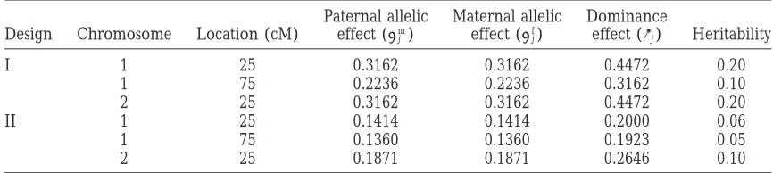
TABLE 1
The true locations and genetic effects of the three simulated QTL
Paternal allelic Maternal allelic Dominance Design Chromosome Location (cM) effect (␣m
j ) effect (␣fj) effect (␦j) Heritability
I 1 25 0.3162 0.3162 0.4472 0.20
1 75 0.2236 0.2236 0.3162 0.10
2 25 0.3162 0.3162 0.4472 0.20
II 1 25 0.1414 0.1414 0.2000 0.06
1 75 0.1360 0.1360 0.1923 0.05
2 25 0.1871 0.1871 0.2646 0.10
The effects are in the scale of liability for the binary data. The heritability is defined as proportion of the variance of liability explained by the locus of interest.
phism of the QTL does not mean anything, although was implemented using an EM algorithm derived byS. Xu(unpublished results).
the four alleles are distinguished. On the other hand,
if the variance is very large, but all four alleles are identi- For all MCMC analyses, the same initial values and priors were used. The initial value for the QTL number cal, we get the equivalent result as zero variance.
There-fore, we decided to control only the variance and let was set at 2 and the corresponding locations were at 50.0 cM of chromosome 1 and 40.0 cM of chromosome the QTL be fully informative. The locations and effects
of the three simulated QTL are given in Table 1. The 2, respectively. The prior Poisson mean of the number of QTL was ⫽2 and the maximum number of QTL value of the liability of each individual took the sum of
the overall mean, values of QTL additive and dominance was L⫽6. The starting values for all regression parame-ters were 0.0. The priors for the regression parameparame-ters effects, and an environmental error sampled from a
standardized normal distribution. The observed binary were normal with mean 0.0 and variance 10.0. The prior for the QTL locations was uniform over the whole ge-phenotype was set to be sj ⫽ 1 if the corresponding
liability exceeds t⫽0, and sj⫽0 otherwise. We designed nome. The tuning parameter of the proposal distribu-tion for QTL locadistribu-tions was chosen to be 2.0 cM. Finally, two simulation experiments. In design I, the overall
mean of the liability was set at 0.0, which generates a the proposal distributions for the allelic and dominance effects were normal with means 0.0 and variance 1.0 in trait incidence of 50%. In design II, the mean was set
at⫺0.95, leading to a trait incidence of 20%. cases where the addition of a new QTL to the model was proposed.
For comparison, the liability of each individual was
also reported and analyzed as if it were observed. There- In each of the MCMC analyses, we ran a single long chain with 106cycles of simulations. The first 200
sam-fore, we analyzed two data sets produced from the same
group of sibs, the binary data and the normally distrib- ples (burn-in period) were discarded and the chain was thinned (saved one iteration in every 50 cycles) to uted data. When the normally distributed data were
analyzed, we used the same program by suppressing the reduce serial correlation in the stored samples so that the total number of samples kept in the analysis was liability-generating subroutine and replacing the
liabili-ties by the reported normal observations. In addition, 2⫻ 104.
we added a subroutine to generate the environmental error because2
εmust be estimated instead of taking a
RESULTS value of unity. The residual variance at each cycle
was updated from its conditional posterior distribution Before we present the result of Bayesian mapping, we first give the results of the ML analysis for the binary p(2
ε|Y, l, , M, Z, ) in the MCMC algorithm. This
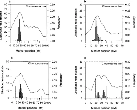
conditional posterior distribution is an inverse gamma data. Figure 1 shows the likelihood profiles along the two chromosomes for both designs. For design I (Figure according to the standard linear model theory when
the prior for2
ε is an inverse gamma distribution (e.g., 1, a and b), we observed one peak at position 26 cM in chromosome 1, overlapping with the true location of the
Gelmanet al. 1995;Sorensen et al. 1995;Satagopan
et al. 1996). For simplicity of programming, however, we first simulated QTL (at 25 cM). The estimated effects of this QTL are␣ˆm
j ⫽0.3744,␣ˆfj⫽0.4024, and␦ˆj⫽0.3858, simply used the Metropolis-Hastings (M-H) algorithm to
generate2εunder a flat prior. very close to the true values. There is no evident peak
in the neighborhood of the second QTL, although the We modified the maximum-likelihood (ML) method
of Xuand Atchley (1996) so that it can handle the test statistics are consistently high. This clearly demon-strates the limitation of the single QTL ML analysis. data with such a full-sib family structure and compared
Figure1.—Likelihood-ratio profiles of ML mapping and empirical distributions of the estimated QTL position obtained by 1000 bootstrap samples from the simulated binary data in design I (a and b) and design II (c and d). The solid curves are the likelihood-ratio profiles and the histograms are the bootstrap frequencies. The left y-axis corresponds to the likelihood-ratio statistic and the right y-axis corresponds to the bootstrap frequency. The true locations of the simulated QTL are indicated with an arrow (↑).
QTL are ␣ˆm
j ⫽ 0.1008, ␣ˆfj ⫽ 0.1654, and ␦ˆj ⫽ 0.3893. estimated QTL locations. We used 1000 bootstrap sam-ples to simulate the distributions of the locations (see One should not expect the estimated values to be
identi-cal to the true values because this only represents the Figure 1). The bootstrap means (the standard devia-tions) are 27.46 (10.08) cM and 25.19 (13.88) cM for result of one random sample with 300 individuals.
For design II (Figure 1, c and d), a major peak was design I, and 24.10 (13.57) cM and 32.2581 (27.71) cM for design II, for the two chromosomes, respectively. observed at 24 cM in chromosome 1 and the
correspond-ing effects were estimated to be ␣ˆm
j ⫽ 0.3193, ␣ˆfj ⫽ In the MCMC analyses, we used the QTL intensity function ofSillanpa¨a¨andArjas(1998, 1999) to detect 0.1873, and ␦ˆj⫽ 0.3230. However, the second QTL in
chromosome 1 remained undetected due to the low the number and locations of QTL. The interval length was chosen to be 1 cM long. The approximate posterior likelihood-ratio value (12.6101). For chromosome 2,
there are two peaks at 25 and 35 cM with the estimated QTL intensities for both the binary and the normal data in design I are shown in Figure 2. The fact that the two effects ␣ˆm
j ⫽ 0.2227,␣ˆjf⫽ 0.2281, and ␦ˆj⫽ 0.1643 and
␣ˆm
j ⫽ 0.1832,␣ˆfj ⫽0.2517, and␦ˆj⫽ 0.1829. Obviously, approximate posterior QTL intensities both have three peaks around the true locations of the three simulated it is difficult to distinguish one QTL or two QTL in
chromosome 2 from the ML analysis. QTL supports a three-QTL model and the true model is indeed of three QTL in design I. Comparing the The ML analyses of QTL mapping do not provide
confidence intervals for the estimated QTL locations shapes of the QTL intensities for the binary and normal data analyses, we can see that binary data analysis does and effects. Confidence intervals would have to be
deter-mined by a resampling technique separately. We lose some information, but the information retained is still sufficient to detect all the simulated QTL.
adopted the bootstrap method of Visscher et al.
in-Figure2.—Histograms of the pos-terior QTL intensity for binary data (top) and normally distributed data (bottom) in design I, respectively. Simulated true QTL locations are in-dicated with an arrow (↑).
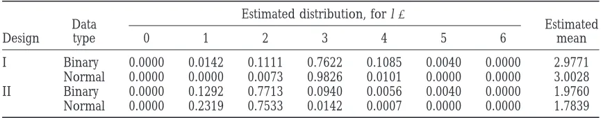
TABLE 2
Empirical posterior distribution of QTL number and the posterior mean
Estimated distribution, for l⫽
Data Estimated
Design type 0 1 2 3 4 5 6 mean
I Binary 0.0000 0.0142 0.1111 0.7622 0.1085 0.0040 0.0000 2.9771 Normal 0.0000 0.0000 0.0073 0.9826 0.0101 0.0000 0.0000 3.0028 II Binary 0.0000 0.1292 0.7713 0.0940 0.0056 0.0040 0.0000 1.9760 Normal 0.0000 0.2319 0.7533 0.0142 0.0007 0.0000 0.0000 1.7839
tensities for both the binary and the normal data in the QTL effects are reliable. As expected, the posterior variances of the normal data are smaller than those design II. For chromosome 1, the QTL intensity graphs
are concentrated around the first QTL locations for obtained for the binary data. For design I, the estimated QTL locations are very close to the corresponding true both the binary and the normal data. The second, the
weakest QTL in chromosome 1, remained undetected values and the standard errors are relatively small com-pared to design II, which has low heritabilities and for both the binary and the normal data, and this result
was practically the same as that obtained from the ML skewed trait incidence. analysis of the binary data in design II. For chromosome
2, the two approximate posterior QTL intensities both
DISCUSSION have one peak and apparently support one QTL
resid-ing at this chromosome. However, the modes of the We have presented here a Bayesian QTL mapping for complex binary traits. The methodology can be gen-intensities for the normal and binary data differ byⵑ9
cM from the simulated true location in chromosome 2. eralized to multiple-ordered categorical traits ( appen-dix c). The most obvious advantage of the Bayesian The approximate posterior distributions for the
num-ber of QTL, obtained from the two designs, are pre- method over existing ML is the ability to investigate the distributions of parameter estimates. Among the sented in Table 2. For design I, the posterior means are
essentially the same for the binary data and the normal parameters of interest, the number of QTL may be the most important one. It is the Bayesian method that data and coincide with the simulated number of QTL.
As expected, the posterior variance of QTL number for provides an easy way to estimate this parameter. The threshold model that the Bayesian mapping is based the normal data is smaller than that for the binary data.
Finally, the posterior mode of the QTL number overlaps on is not new to QTL mapping for categorical traits. Bayesian mapping for normally distributed traits is also with the true number for both types of data in design
I. In the analysis of design II, the estimated posterior available. In this article we combine both techniques to develop the Bayesian mapping for binary traits. The distributions for the number of QTL appear to have
shifted to the left by 1 compared with the simulated main point of the threshold model is that by introducing an underlying normal variable into the problem, the number of QTL, for the two types of data. Again, as in
design I, the posterior means and modes are essentially binary response is connected to the normal linear model via the probit function. The major advantage of the thresh-the same for both thresh-the binary data and thresh-the normal data.
Consider next the estimations of QTL effects. The old model as applied to Bayesian mapping is that once the underlying liability is generated, all other unknowns estimates are reliable only in chromosome regions in
which the posterior QTL intensity or the posterior den- have conditional posterior distributions identical to those already given in Bayesian analysis of normal data. sity of QTL locations is sufficiently high (Sillanpa¨a¨
andArjas1998, 1999;StephensandFisch1998). The Since the liability is a hypothetical variable, the inter-pretation of categorical data with a threshold model highest posterior region attempts to capture a
compara-tively small region of the parameter space that contains can be delicate. However, there are a number of ways to test the general validity of the model (Lynch and most of the posterior probability mass. The
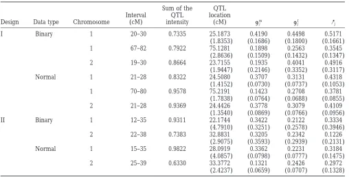
chromo-some regions with sufficiently high posterior QTL inten- Walsh1998, Chapter 25). In the threshold model, the liability is usually assumed normal. In reality, the nature sity are given in Table 3. We used only the posterior
samples, in which QTL locations fall into the regions of the underlying variable is always unknown. In Bayes-ian analysis, some kind of distribution must be assigned described in Table 3, to estimate the QTL effects. The
posterior distributions of the QTL effects are presented to this hypothetical variable and normal distribution is the natural choice. In addition, Tan et al. (1999) re-graphically in Figure 4 for the three identified QTL for
design I. The point estimates and the estimation errors cently showed that the normal assumption for the liabil-ity is robust to obvious departure from normalliabil-ity. of locations and effects of QTL for the two designs are
infer-TABLE 3
The highest posterior QTL intensity interval, Bayesian estimates of QTL locations, and allelic and dominance effects
Sum of the QTL Interval QTL location
Design Data type Chromosome (cM) intensity (cM) ␣m
j ␣fj ␦j
I Binary 1 ⵑ20–30 0.7335 25.1873 0.4190 0.4498 0.5171
(1.8353) (0.1686) (0.1800) (0.1661) 1 ⵑ67–82 0.7922 75.1281 0.1898 0.2563 0.3545
(2.8636) (0.1509) (0.1432) (0.1347) 2 ⵑ19–30 0.8664 23.7155 0.1935 0.4041 0.4916
(1.9447) (0.2146) (0.3352) (0.3117)
Normal 1 ⵑ21–28 0.8322 24.5080 0.3707 0.3131 0.4318
(1.4152) (0.0730) (0.0737) (0.1053) 1 ⵑ70–80 0.9578 75.2191 0.1423 0.2708 0.3781
(1.7838) (0.0764) (0.0688) (0.0855) 2 ⵑ21–28 0.9369 24.4426 0.3778 0.3079 0.4109
(1.3540) (0.0869) (0.0766) (0.0956)
II Binary 1 ⵑ12–35 0.9311 22.1744 0.3422 0.2122 0.3334
(4.7910) (0.3251) (0.2578) (0.3946) 2 ⵑ22–38 0.7383 32.8831 0.3205 0.2342 0.1226
(2.9075) (0.3593) (0.2939) (0.2131)
Normal 1 ⵑ15–35 0.9822 28.0919 0.3362 0.2231 0.3184
(4.0857) (0.0798) (0.0777) (0.1475) 2 ⵑ25–39 0.6330 33.3772 0.1321 0.2426 0.2972
(2.4237) (0.0659) (0.0707) (0.1328)
Posterior standard errors of the estimates are given in parentheses.
ences about the number of QTL, their locations, and levels of randomness and the resultant ability to com-bine information from different sources. Therefore, the effects. There are a number of advantages in arriving
at inferential statements by using a Bayesian approach Bayesian approach could be extended to allow more complicated models for more complicated data struc-over the traditional methods. First, Bayes’ method
pro-vides a complete posterior distribution for the number tures.
An essential element of our full Bayesian mapping of QTL, their locations, and the corresponding effects.
As a consequence, interval estimates of the parameters for binary traits is its ability to move between different values of the QTL number. The proposed method per-can be obtained straightforwardly. In contrast, ML only
produces point estimates of these parameters. Confi- formed well for the simulated data. The mixing property of the MCMC algorithm does not seem to be overly dence intervals would have to be determined separately,
for example, by employing bootstrap (Visscher et al. sensitive to the choice of the initial values of the un-knowns. For example, when we started with l0⫽6, after
1996b) or other sampling-based methods. Second, it is
usually difficult to determine the correct number of 100 iterations l quickly dropped to 3 and subsequently behaved the same as when we started with l0 ⫽ 2. A
QTL using traditional methods. It has been shown that
an incorrect specification for the number of QTL can similar conclusion has been obtained byHeath(1997). However, the mixing property seems to be greatly af-lead to distortion of estimates of locations and effects
when ML and least squares (LS) are used. Bayesian fected by the proposal distribution for QTL effects when a new QTL is added to the model. Therefore, this pro-mapping allows one to include the number of QTL as an
unknown in the analysis and thus avoids this distortion. posal distribution should be chosen with care (Heath
1997;StephensandFisch1998;Sillanpa¨a¨andArjas
Third, a common problem with traditional methods
is how to choose the appropriate critical value of the 1999). To ensure sufficient mixing, the single MCMC chain must be sufficiently long. Although the method statistical test for declaration of the presence of QTL.
With the reversible jump MCMC, the number and the is computationally very intensive, it does not need re-peated analyses of resampled data, as required in ML locations of QTL can be characterized by the posterior
probability distribution of the number of QTL and the for the permutation test. On a Sun SPARC 5 workstation, our analyses with a MCMC chain of 106 took ⵑ6.5 hr
posterior QTL intensity. One can even calculate the
posterior probability that some particular chromosomal for normal data and 8 hr for binary data, respectively. A major implementation issue in MCMC is to determine region contains at least one QTL (Sillanpa¨a¨andArjas
Figure4.—Approximate posterior distributions of maternal allelic effects (␣f
j), paternal allelic effects (␣fj), and dominance effects (␦j) for j⫽1, 2, 3, for design I. Simulated true values of QTL effects are indicated with an arrow (↑). The solid curves represent QTL mapping for binary data: (a) the first QTL determined from interval ⵑ20–30 cM of chromosome 1; (b) the second QTL determined from intervalⵑ67–82 cM of chromosome 1; (c) the QTL on chromosome 2 determined from interval
ⵑ19–30 cM. The dotted curves represent QTL mapping for normal data: (a) the first QTL determined from interval ⵑ21–28 cM of chromosome 1; (b) the second QTL determined from intervalⵑ70–80 cM of chromosome 1; (c) the QTL on chromosome 2 determined from intervalⵑ21–28 cM.
serial correlation between the samples, and the burn- the offspring. If grandparents are also genotyped, the linkage phases can be accurately reconstructed; other-in period. When analyzother-ing real data, one can examother-ine
time series graphs of simulated sequence and calculate wise, a relatively large number of offspring for each family are required (Knottet al. 1996). Alternatively, the Monte Carlo variance to obtain estimates of the
effective sample sizes of all parameters (Geyer1992). one can treat linkage phases as random variables in the Bayesian analysis, as done bySillanpa¨a¨andArjas
In our simulation studies, it is difficult to calculate series
correlation because the dimension keeps changing from (1999). When the family size is too small, inference of the parental linkage phases will be subject to large error one cycle to another. When the dimension changes,
the identities of the QTL also change. Therefore, we and stochastic resampling is certainly required. When the mapping population contains many small families, empirically determined the burn-in period, the length
of the MCMC chain, and the interval length of subsam- accurate inferences of parental linkage phases are al-most impossible and other statistical models may be pling to reduce the serial correlation.
The Bayesian procedure presented in this study is considered, such as the IBD-based random model ap-proach (Xu and Atchley 1995). Under the random based on known marker linkage phases in the parents.
When the linkage phases are not known, they must be model approach, one does not need to know the num-ber of alleles and the parental linkage phases.
As an alternative to the approach of the liability aug- LITERATURE CITED
mentation, one can directly use the probit relationship Albert, J. H.,andS. Chib,1993 Bayesian analysis of binary and
polychotomous response data. J. Am. Stat. Assoc. 88: 669–679.
between the binary phenotype and the model effects to
Churchill, G. A.,andR. W. Doerge,1994 Empirical threshold
simulate the model effects by using the
Metropolis-values for quantitative trait mapping. Genetics 138: 963–971.
Hastings algorithms, i.e., replacing Devroye, L.,1986 Non-Uniform Random Variable Generation.
Springer-Verlag, New York.
Falconer, D. S.,andT. F. C. Mackay,1996 Introduction to Quantita-p(S|Y, l,, Z,)p(Y|l,, Z, )
tive Genetics, Ed. 4. Longman, London.
Gelfand, A. E., and A. F. M. Smith, 1990 Sampling-based
ap-by proaches to calculating marginal densities. J. Am. Stat. Assoc. 85:
398–409.
p(S|l,, Z,)⫽
冮
Yp(S|Y, l,, Z,)p(Y|l,, Z,)d Y. Gelman, A., J. B. Carlin, H. S. SternandD. B. Rubin,1995
Bayes-ian Data Analysis. Chapman & Hall, London.
Geyer, C. J.,1992 Practical Markov chain Monte Carlo. Stat. Sci. 7:
In the simple situation, such as a single line cross or full- 473–511.
Green, P. J.,1995 Reversible jump Markov chain Monte Carlo
com-sib family, application of the probit model is poscom-sible. In
putation and Bayesian model determination. Biometrika 82: 711–
fact, it will improve the mixing property of the MCMC
732.
because the unobserved liability has been integrated Hackett, C. A.,andJ. I. Weller,1995 Genetic mapping of
quantita-tive trait loci for traits with ordinal distributions. Biometrics 51:
out. We decided to utilize the data augmentation
ap-1252–1263.
proach by generating the liability because the method Haley, C. S.,andS. A. Knott,1992 A simple regression method can be easily extended to more complicated situations, for mapping quantitative trait loci in line crosses using flanking
markers. Heredity 69: 315–324.
such as mapping for ordered categorical data or
multi-Heath, S. C.,1997 Markov chain Monte Carlo segregation and
ple traits. linkage analysis for oligogenic models. Am. J. Hum. Genet. 61: As mentioned previously, the major advantage of 748–760.
Hoeschele, I.,andP. VanRanden,1993a Bayesian analysis of
link-Bayesian mapping is the ability to handle multiple QTL
age between genetic markers and quantitative trait loci. I. Prior
with multiple effects, including epistatic effects. Epi- knowledge. Theor. Appl. Genet. 85: 953–960.
Hoeschele, I.,andP. VanRanden,1993b Bayesian analysis of
link-static effects can be important in phenotypic evolution.
age between genetic markers and quantitative trait loci. II.
Com-Although we did not add the epistatic effects in our
bining prior knowledge with experimental evidence. Theor. Appl.
Bayesian model presented in this study, it is not difficult Genet. 85: 946–952.
Jansen, R. C.,1993 Interval mapping of multiple quantitative trait
to do so. When a new QTL is proposed, its interactive
loci. Genetics 135: 205–211.
effects with all existing QTL should be proposed and, Jansen, R. C., D. L. JohnsonandJ. A. M. Van Arendonk,1998 A if accepted, the epistatic effects should be included in mixture approach to the mapping of quantitative trait loci in complex populations with an application to multiple cattle
fami-the model. A QTL is finally added to fami-the model if at
lies. Genetics 148: 391–399.
least one effect caused by the QTL is accepted. This will Kao, C. H., Z.-B. ZengandR. D. Teasdale,1999 Multiple interval involve additional reversible jumps on the dimension mapping for quantitative trait loci. Genetics 152: 1203–1216.
Knott, S. A., J. M. ElsenandC. S. Haley,1996 Methods for
multi-of the model even if the number multi-of QTL remains the
ple-marker mapping of quantitative trait loci in half-sib
popula-same. tions. Theor. Appl. Genet. 93: 71–80.
Kruglyak, L.,andE. S. Lander,1995 A nonparametric approach
Throughout the study, we update the genotype
indi-for mapping quantitative trait loci. Genetics 139: 1421–1428.
vidual by individual and locus by locus. In general, this
Lander, E. S.,andD. Botstein,1989 Mapping Mendelian factors
kind of single-site update does not always lead to an underlying quantitative traits using RFLP linkage maps. Genetics 121:185–199.
irreducible sampler because of strong dependency of
Lynch, M.,andB. Walsh,1998 Genetics and Analysis of Quantitative close relatives and strong dependency of adjacent loci. Traits. Sinauer Associates, Sunderland, MA.
In practice, when we deal with complicated pedigree Rao, S.,andS. Xu,1998 Mapping quantitative trait loci for ordered categorical traits in four-way crosses. Heredity 81: 214–224.
data and closely linked markers, block updating more
Rebai, A.,1997 Comparison of methods for regression interval
map-than one individual and more map-than one locus is required ping in QTL analysis with non-normal traits. Genet. Res. 69:
69–74.
for appropriate mixing of the sampler (e.g., Heath
Richardson, S., andP. J. Green, 1997 On Bayesian analysis of
1997;Sillanpa¨a¨andArjas1999). In our study, because
mixtures with an unknown number of components. J. R. Stat.
the pedigree is simple and the marker loci are not close Soc. Ser. B 59: 731–792.
Satagopan, J. M.,andB. S. Yandell,1996 Estimating the number
enough, we did not find any insufficient mixing in
geno-of quantitative trait loci via Bayesian model determination.
Spe-type sampling. A Bayesian mapping for complicated cial Contributed Paper Session on Genetic Analysis of Quantita-pedigree data is now under investigation in this labora- tive Traits and Complex Diseases, Biometric Section, Joint
Statisti-cal Meeting, Chicago.
tory, where a block updating strategy is being
incorpo-Satagopan, J. M., B. S. Yandell, M. A. NewtonandT. C. Osborn, rated in the sampler. 1996 A Bayesian approach to detect quantitative trait loci using
Markov chain Monte Carlo. Genetics 144: 805–816. We thank Dr. D. D. Gessler for his helpful comments on the
manu-Sillanpa¨a¨, M. J.,andE. Arjas,1998 Bayesian mapping of multiple script. We also thank two anonymous reviewers for their critical
com-quantitative trait loci from incomplete inbred line cross data. ments on an earlier version of the manuscript. This research was Genetics 148: 1373–1388.
supported by the National Institutes of Health Grant GM55321-03 Sillanpa¨a¨, M. J.,andE. Arjas,1999 Bayesian mapping of multiple and the U.S. Department of Agriculture National Research Initiative quantitative trait loci from incomplete outbred offspring data.
Sorensen, D. A., S. Andersen, D. GianolaandI. Korsgaard,1995 coefficients:Given the liability Y, the number l, and the Bayesian inference in threshold models using Gibbs sampling.
genotype Z of QTL, the posterior distribution for
Genet. Sel. Evol. 27: 229–249.
Stephens, D. A.,andR. D. Fisch,1998 Bayesian analysis of quantita- can be derived using the standard normal linear model
tive trait locus data using reversible jump Markov chain Monte theory. If normal priors are chosen for the regression Carlo. Biometrics 54: 1334–1347.
coefficients, these posterior distributions are given by Tan, M., Y. QuandJ. S. Rao,1999 Robustness of the latent variable
model for correlated binary data. Biometrics 55: 258–263.
k|Y, l, Z, {j}j⬆k,␥ Tanner, M. A.,andW. H. Wong,1987 The calculation of posterior
distributions by data augmentation. J. Am. Stat. Assoc. 82: 528– 549.
ⵑN
冢
0k/2 k⫹
兺
n
i⫽1xik(yi⫺XTi ⫺
兺
lj⫽1ZTijH␥i⫹xikk) 1/2k⫹
兺
n i⫽1x2ik, Thaller, G.,andI. Hoeschele,1996 A Monte Carlo method for
Bayesian analysis of linkage between single markers and quantita-tive trait loci: I. Methodology. Theor. Appl. Genet. 93: 1161–1166.
Uimari, P.,andI. Hoeschele,1997 Mapping linked quantitative 1
1/2 k⫹
兺
n i⫽1x2ik
冣
, (A3)
trait loci using Bayesian method analysis and Markov chain Monte Carlo Algorithms. Genetics 146: 735–743.
Uimari, P., G. ThallerandI. Hoeschele,1996 The use of multiple markers in a Bayesian method for mapping quantitative trait loci.
for k⫽1, · · · , p. Each of the allelic effects has a normal
Genetics 143: 1831–1842.
posterior distribution, Visscher, P. M., C. S. HaleyandS. A. Knott,1996a Mapping QTL
for binary traits in backcross and F2populations. Genet. Res. 68:
55–63. ␣v
j *|Y, l, Z,, {␥j}j⬆j*,␣vj *,␦j *
Visscher, P. M., R. ThomsonandC. S. Haley,1996b Confidence intervals in QTL mapping by bootstrapping. Genetics 143: 1013–
ⵑN
冢冤
␣v 0j *
2
␣v j *
⫹兺n
i⫽1 (ZT
ij *Hv)[yi⫺XTi ⫺兺 l
j⫽1 ZT
ijH␥j⫹(ZTij*Hv)␣vj *]
冥
/冤
1
2
␣v j *
⫹兺n
i⫽1 (ZT
ij *Hv)2
冥
, 1020.Xu, S.,andW. R. Atchley,1995 A random model approach to interval mapping of quantitative trait loci. Genetics 141: 1189–
1/
冤
12␣v j *
⫹兺n
i⫽1
(ZTij *Hv)2
冥冣
, (A4)1197.
Xu, S.,andW. R. Atchley,1996 Mapping quantitative trait loci for complex binary diseases using line crosses. Genetics 143:
where v⫽ m, s and
1417–1424.
Xu, S., N. Yonash, R. L. VallejoandH. H. Cheng,1998 Mapping quantitative trait loci for complex binary traits using a
heteroge-v⫽
m if v⫽ f
f if v⫽m.
neous residual variance model: an application to Marek’s disease susceptibility in chickens. Genetica 104: 171–178.
Yi, N.,andS. Xu,1999a Mapping quantitative trait loci for complex
The posterior distribution of the dominance effect is
binary traits in outbred populations. Heredity 82: 668–676.
Yi, N.,andS. Xu,1999b A random approach to mapping quantitative
␦j *|Y, l, Z,, {␥j}j⬆j *,␣mj *,␣fj * trait loci for complex binary traits in outbred populations.
Genet-ics 153: 1029–1040.
Zeng, Z.-B.,1994 Precision mapping of quantitative trait loci. Genet- ⵑN
冢
␦0j *2
␦j *
⫹兺n
i⫽1 (ZTij *H
␦)[yi⫺XTi ⫺兺 l
j⫽1 ZijHT ␥
j⫹(ZTij *H␦)␦j *]
冥
/冤
1
2
␦j *
⫹兺n
i⫽1 (ZTij *H
␦)2
冥
,ics 136: 1457–1468.
Communicating editor:T. F. C. Mackay
1/
冤
12
␦j *
⫹兺n
i⫽1 (ZTij *H
␦)2
冥冣
, (A5) for j*⫽ 1, · · · , l, where0k,␣0j *m ,␣f0j *, and␦0j *are theAPPENDIX A: CONDITIONAL prior means for k, ␣mj *, ␣fj *, and ␦j *, respectively, and POSTERIOR DISTRIBUTIONS 2
k,
2
␣m
j *,
2
␣f
j *, and ␣
2
␦j * are the prior variances for k,
␣m
j *,␣fj *, and␦j *. Conditional posterior distribution of the liability yi:
Conditional posterior distributions of the QTL and Conditional on , Zi, and si, the liability yi follows a
marker genotypes: The conditional posterior distribu-truncated normal distribution. Depending on the
bi-tion of the QTL genotype Zij is a discrete distribution nary phenotypic value si, we have
over the possible genotypes. In model (1), the QTL genotype Zijtakes one of four values. Thus, for instance, p(yi|, Zi,si⫽1)⫽
(yi⫺XTi ⫺
兺
lj⫽1ZTijH␥j, 1) ⌽(XTi ⫹
兺
lj⫽1ZTijH␥j)1(yi⬎0)
the conditional posterior distribution that an individual (A1) takes a genotype z
ij⫽(1, 0, 0, 0)Tis given by
p(Zij⫽ zij|yi,, Zi(⫺j), Mi,) and
⫽ p(yi|, Zij ⫽zij, Zi(⫺j),)p(Zij⫽zij|j, Zlij, Zrij)
兺
Zijp(yi|, Zij, Zi(⫺j),)p(Zij|j, Zl
ij, Zrij) , p(yi|, Zi,si⫽0)⫽
(yi⫺XTi ⫺
兺
lj⫽1ZTijH␥j, 1) 1⫺ ⌽(XTi ⫹
兺
lj⫽1ZTijH␥j)1(yiⱕ0),
(A2) (A6)
where Zi(⫺j) ⫽ {Zij⬘ : 1 ⱕ j⬘ ⱕ l, j⬘⬆ j }, and Zlij (Zrij) is where (x, 2) is the normal density with mean zero
and variance 2 and ⌽(·) is the standardized normal the left (right) flanking genotype of the jth QTL of the
ith individual (markers or QTL). distribution function.
APPENDIX C: GENERALIZATION TO MULTIPLE-genotype Mij is dependent only on the genotypes of
ORDERED CATEGORICAL TRAITS relevant flanking loci (marker or QTL). Taking the
prior of the marker into consideration, we can obtain The method described in the text can be generalized to multiple-ordered categorical traits. Suppose now that p(Mij⫽mij|Mlij, Mrij)⫽
p(Mij⫽ mij)p(Mlij, Mrij|Mij⫽mij) p(Ml
ij, Mrij)
, the observed phenotypic value sitakes one of c ordered categories, 1, · · · , c. A set of fixed thresholds, t1⬍t2⬍
(A7)
· · · ⬍ tc⫺1, in the scale of the liability determine the
observed categories. Let t0 ⫽ ⫺∞ and tc ⫽ ⫹∞. We where Ml
ij (Mrij) is the left (right) flanking complete
observe si, where si⫽k if tk⫺1 ⬍yiⱕtk(k⫽ 1, · · ·, c). genotype of the jth marker of the ith individual, and
The thresholds t1, · · ·, tc⫺1 are unknown and need to
p(Mij ⫽ mij) is the prior probability of the jth marker
be estimated. To ensure that the parameters are identi-of the ith individual. p(Mij ⫽ mij) is calculated by the
fiable, it is necessary to impose one restriction on the multipoint method (RaoandXu 1998).
thresholds. Without loss of generality, we take t1 ⫽ 0
(Albert and Chib 1993) and estimate t ⫽ (t2, · · · ,
tc⫺1). Assuming that t and (l, , ) are independently
APPENDIX B: ACCEPTANCE PROBABILITIES
distributed a priori, the joint posterior distribution can Updating QTL locations: To modify the location j
be written as of the jth QTL, a proposal jnew is generated from a
uniform distribution on the interval [j⫺ d, j ⫹ d], p(Y, l,, M, Z,, t|S)⬀p(S|Y, l,, Z,, t)p(Y|l,, Z,) where d is a tuning parameter. The acceptance
probabil-⫻ p(Z|l,, M)p(M)p(l, ,)p(t), (C1) ity for the change fromjtojnewtakes min{1,␣}, where
the relative importance ratio␣is defined as
where p(Y|l,, Z,), p(Z|l,, M), p(M), and p(l,, ) are the same as for the binary data model. The first
␣ ⫽p(Y, l,newj ,⫺j, M, Z,|S) p(Y, l,j,⫺j, M, Z,|S)
⫽
兿
ni⫽1
p(Zij|newj , Zl*ij, Zr*ij) p(Zij|j, Zlij, Zrij)
, term in (C1) is the likelihood and expressed as (Albert
andChib1993;Sorensenet al. 1995) (B1)
where ⫺j ⫽ {j⬘ : 1 ⱕ j⬘ ⱕ l, j⬘ ⬆ j}, Zlij (Zrij) is the p(Y|l,, Z,)⫽
兿
ni⫽1
兺
c
k⫽1
1(tk⫺1⬍ yi ⱕtk)1(si⫽k)
.
genotype of the left (right) flanking locus (marker or
(C2) QTL) at the current position for the jth QTL in the ith
individual, and Zl*
ij(Zr*ij) is the genotype of the left (right)
The last term in (C1), p(t), is the prior density of t and flanking locus at the proposed new location for the jth
is discussed below. QTL in the ith individual.
It is clear that the conditional posterior distributions Add one new QTL: Given the liability Y, the
accep-of, M, and Z are the same as those specified in the tance probability is the same as that of the normal trait,
binary model. For the liability associated with the kth except that the normal observables are replaced by the
observation, we have simulated values of liability. As inSillanpa¨a¨andArjas
(1998), the acceptance probability is min{1,␣}, where
p(yi|, Zi, si⫽k)
␣ ⫽exp{⫺1⁄2
兺
ni⫽1(yi⫺XTi ⫺兺
lj⫽1ZTijH␥j⫺Z*iTH␥*)2} exp{⫺1⁄2
兺
ni⫽1(yi⫺XTi ⫺兺
lj⫽1ZTijH␥j)2} ⫽(yi⫺XTi ⫺
兺
jl⫽1ZTijH␥j, 1)⌽(tk⫺XTi ⫺
兺
lj⫽1ZTijH␥j)⫺ ⌽(tk⫺1⫺XTi ⫺
兺
l j⫽1ZTijH␥j)1
(tk⫺1⬍yiⱕtk), (C3)
⫻ l⫹1⫻
pd
(l⫹1)pa
, (B2)
where(x,2) stands for the normal density with mean
where Z*i is the proposed genotype of the ith individual, 0 and variance2, and⌽(·) is the standardized normal
␥* are the proposed QTL effects, and is the prior distribution function. If we assign a diffuse prior for t, mean of the QTL number. the conditional posterior distribution of t
kgiven {tj, j⬆ Delete one QTL:If the jth existing QTL is proposed
k} and all the other parameters is uniform on the interval to be removed from the model, the acceptance
probabil-[max{max{yi: si⫽k}, tk⫺1}, min{min{yi: si⫽k⫹1}, tk⫹1}]
ity is min{1,␣}, where
(AlbertandChib 1993;Sorensenet al. 1995). The MCMC algorithm for the binary case described
␣ ⫽exp{⫺1⁄2
兺
ni⫽1(yi⫺XTi ⫺兺
l
j⬘⬆jZTij⬘H␥j⬘)2} exp{⫺1⁄
2
兺
ni⫽1(yi⫺XTi ⫺兺
lj⫽1ZTijH␥j)2}⫻ l
⫻
lpa
pd
. in the text is now generalized to multiple-ordered cate-gorical traits. In brief, we only need to modify the likeli-(B3)
hood and generated t. Eventually, the liability is gener-ated according to a doubly truncgener-ated normal rather In (B2) and (B3), the first term is the likelihood ratio,
than a singly truncated one. Updating of other parame-the second term is parame-the prior ratio, and parame-the third term