ABSTRACT
LI, XIAOSHAN. Tensor Based Statistical Models with Applications in Neuroimaging Data Analysis. (Under the direction of Dr. Lexin Li and Dr. Hua Zhou.)
In the last few years there has been growing interest in neuroimaging data analysis. Large-scale neuroimaging studies have been collecting images of study individuals, which take the form of two-dimensional, three-dimensional, or higher dimensional arrays, also known as tensors. Addressing scientific questions arising from such data demands new statistical models that take multidimensional arrays as covariates, which further add complications to dimension reduction problems. In this dissertation, we study methods of statistical modeling when covariates are multidimensional arrays. There are three parts in this dissertation.
In the first part (Chapter 2), we propose a family of generalized linear tensor re-gression models based upon the Tucker decomposition of rere-gression coefficient arrays. Effectively exploiting the low rank structure of tensor covariates brings the ultra-high dimensionality to a manageable level that leads to efficient estimation. We demonstrate the new model could both numerically provide a sound recovery of even high rank sig-nals and asymptotically estimate the best Tucker structure approximation to the full array model. Simulation studies and real data analysis show that the proposed Tucker model outperforms a recently proposed CANDECOMP/PARAFAC (CP) tensor regres-sion model.
classical method to handle measurement error model.
©Copyright 2014 by Xiaoshan Li
Tensor Based Statistical Models with Applications in Neuroimaging Data Analysis
by Xiaoshan Li
A dissertation submitted to the Graduate Faculty of North Carolina State University
in partial fulfillment of the requirements for the Degree of
Doctor of Philosophy
Statistics
Raleigh, North Carolina 2014
APPROVED BY:
Dr. Arnab Maity Dr. Ana-Maria Staicu
Dr. Lexin Li
Co-chair of Advisory Committee
Dr. Hua Zhou
DEDICATION
BIOGRAPHY
ACKNOWLEDGEMENTS
I would like to express my sincerest gratitude and appreciation to my advisors, Dr. Lexin Li and Dr. Hua Zhou, for their immense help in the entire journey of my research career at NCSU. Their insightful instruction, generous support and unending encouragement guided me throughout every step of my research. The experience of working with them has been great, and I have learned a lot from my advisors, not only on specific statistical knowledge, but the professional attitudes and activities in research work as well.
I thank Dr. Arnab Maity for the valuable guidance he provided at the early stage of my research, and for joining my thesis committee. His valuable advice helped expand my horizons in statistics research in the first two years of study at NCSU. I thank all the other members in my thesis committee, Dr. Ana-Maria Staicu and Dr. Kara Peters, for carefully reviewing this thesis and providing valuable suggestions.
I am grateful to all the faculty members in the department for offering a comprehensive collection of courses in statistics, which help lay solid foundations for my research. I would like to thank Dr. Charlie Smith for his warm greetings and snacks when I stay up late in the Lab. Also I would like to thank all the staff for their excellent service to the department, which creates great environment for study.
I also owe my gratitude to my mentors, Jeffery Painter and Alan Menius, at Glaxo-SmithKline Pharmaceutical, where I worked as a Graduate Industrial Traineeship, and David Grinder at American Credit Acceptance, where I worked as an internship. Under their instruction, I got access to statistical methods used in real industrial applications. Thanks to my fellow students and friends at NCSU. Your supports and encourage-ments have made my life easier and enriched my life in the United States.
TABLE OF CONTENTS
LIST OF TABLES . . . ix
LIST OF FIGURES . . . xi
Chapter 1 Introduction . . . 1
1.1 Overview of Brain Imaging Analysis . . . 1
1.2 Tensor Decomposition Preliminaries . . . 4
1.3 Thesis Organization . . . 6
Chapter 2 Tucker Tensor Regression and Neuroimaging Analysis . . . . 9
2.1 Introduction . . . 9
2.2 Overview . . . 13
2.3 Literature Review – Application of Tucker . . . 14
2.4 Model . . . 15
2.4.1 Tucker Tensor Decomposition Preliminaries . . . 15
2.4.2 Tucker Regression Model . . . 15
2.4.3 Duality and Tensor Basis Pursuit . . . 17
2.4.4 Model Size: Tucker vs CP . . . 17
2.5 Estimation . . . 20
2.6 Statistical Theory . . . 23
2.6.1 Score and Information . . . 23
2.6.2 Identifiability . . . 26
2.6.3 Asymptotics . . . 28
2.7 Regularized Estimation . . . 29
2.8 Numerical Study . . . 31
2.8.1 Identification of Various Shapes of Signals . . . 31
2.8.2 Comparison of the Regularized Tucker and Standard Statistical Models . . . 32
2.8.3 Performance with Increasing Sample Size . . . 34
2.8.4 Comparison of the Tucker and CP Models . . . 36
2.8.5 Attention Deficit Hyperactivity Disorder Data Analysis . . . 38
2.9 Discussion . . . 42
2.9.1 Summary . . . 42
2.9.2 Computation Time . . . 43
2.9.3 Limitation . . . 44
Chapter 3 Tensor Regression with Measurement Error . . . 45
3.1 Introduction . . . 45
3.3 Notations . . . 47
3.3.1 Classical Setup . . . 47
3.3.2 Tensor Setup . . . 48
3.4 Literature Review . . . 49
3.4.1 Functional Model . . . 49
3.4.2 Regression Calibration . . . 52
3.4.3 SIMEX . . . 54
3.4.4 Conditional Score . . . 56
3.4.5 Instrumental Variables . . . 57
3.5 Model – Vector X . . . 60
3.5.1 Review of Conditional Score Method . . . 60
3.5.2 Extension of Conditional Score Equation . . . 62
3.5.3 Conversion to Optimization Problem . . . 66
3.6 Model – Tensor X . . . 67
3.6.1 Optimization – Linear Regression . . . 68
3.6.2 Optimization – Logistic Regression . . . 71
3.7 Numerical Study . . . 71
3.7.1 Simulation Setup . . . 72
3.7.2 Simulation Results . . . 73
3.8 Discussion . . . 74
3.8.1 Summary . . . 74
3.8.2 Computation Time . . . 79
3.8.3 Limitation . . . 79
Chapter 4 Tensor Linear Support Vector Machines . . . 81
4.1 Introduction . . . 81
4.2 Overview . . . 82
4.3 Literature Review . . . 83
4.3.1 Feature Selection . . . 83
4.3.2 Dimension Reduction Methods . . . 91
4.3.3 Classification Models . . . 97
4.4 Model and Optimization . . . 99
4.4.1 Introduction to Support Vector Machine (SVM) . . . 99
4.4.2 Tensor Linear SVM . . . 101
4.5 Numerical Study . . . 104
4.5.1 Example 1 . . . 104
4.5.2 Example 2 . . . 106
4.5.3 EEG Data Analysis . . . 109
4.6 Discussion . . . 113
4.6.1 Summary . . . 113
4.6.3 Limitation . . . 114
References . . . 115
Appendices . . . 130
Appendix A Proofs in Chapter 2 . . . 131
A.1 Proof of Lemma 2 . . . 131
A.2 Proof of Proposition 1 . . . 132
A.3 Proof of Lemma 3 . . . 133
A.4 Proof of Proposition 2 . . . 135
A.5 Proof of Proposition 3 . . . 136
A.6 Proof of Theorem 1 . . . 136
Appendix B Proofs in Chapter 3 . . . 138
B.1 Derivation of (3.10) . . . 138
LIST OF TABLES
Table 2.1 Number of free parameters in Tucker and CP models. . . 19 Table 2.2 Comparison of regularized Tucker model with LASSO penalty (R-Tucker),
vectorizedν-SVM regression model (V-ν-SVM) and vectorized regular-ized linear regression model with LASSO penalty (V-GLM) in terms of root mean squared error (RMSE) of B Estimate. Results are averaged over 100 replications. Numbers in parentheses are standard errors . . . 34 Table 2.3 Comparison of the Tucker and CP models. Reported are the average
and standard deviation (in the parenthesis) of the root mean squared error, all based on 100 data replications. . . 38 Table 2.4 ADHD testing data misclassification error. . . 40 Table 2.5 ADHD model fitting run time (in seconds). . . 42 Table 2.6 Fitting run time for recovering ‘triangle’ shape (in seconds) at rank 1,
2, 3 and 4. Reported are the median time of 100 runs. . . 43 Table 2.7 Computing time comparison of the Tucker and CP models in Section
2.8.4. Reported are median time (in seconds) over 100 runs. . . 43 Table 3.1 Mean Absolute Error (MAE) of B estimate for ‘T’ shape in linear and
logistic regression. The true regression coefficient for each entry is either 0 or 1. The matrix variate has size 32 by 32 with entries generated as standard normals. The estimate is averaged over 100 data replicates. . 75 Table 3.2 Mean Absolute Error (MAE) of B estimate for ‘cross’ shape in linear
and logistic regression. The true regression coefficient for each entry is either 0 or 1. The matrix variate has size 32 by 32 with entries generated as independent standard normals. The estimate is averaged over 100 data replicates. . . 76 Table 3.3 Mean Absolute Error (MAE) ofBestimate for ‘disk’ shape in linear and
logistic regression. The true regression coefficient for each entry is either 0 or 1.The matrix variate has size 32 by 32 with entries generated as independent standard normals. The estimate is averaged over 100 data replicates. . . 77 Table 3.4 Mean Absolute Error (MAE) of B estimate for ‘pentagon’ shape in
linear and logistic regression. The true regression coefficient for each entry is either 0 or 1. The matrix variate has size 32 by 32 with entries generated as independent standard normals. The estimate is averaged over 100 data replicates. . . 78 Table 3.5 Fitting run time for ‘cross’ shape (in seconds) at rank 2, 3 and 4 in
Table 3.6 MAE of β estimate in classical setup (vector case). Sample size is 500. The estimate is averaged over 100 data replicates. . . 80 Table 4.1 Comparison of tensor SVM (tsvm), linear SVM (lsvm), radial kernel
SVM (rsvm), and tensor logistic regression with L1 and L2 regular-ization (glm(L1),glm(L1)) in terms of misclassification rate in linear learning setup. Results are averaged over 100 replications. Numbers in parentheses are standard errors. . . 105 Table 4.2 Comparison of tensor SVM (tsvm), linear SVM (lsvm), radial kernel
SVM (rsvm), and tensor logistic regression with L1 and L2 regulariza-tion (glm(L1),glm(L2)) in terms of misclassification rate in logit link setup. Results are averaged over 100 replications. Numbers in paren-theses are standard errors. . . 107 Table 4.3 Comparison of tensor SVM (tsvm), linear SVM (lsvm), radial kernel
SVM (rsvm), and tensor logistic regression with L1 and L2 regulariza-tion (glm(L1),glm(L2)) in terms of misclassification rate in probit link setup. Results are averaged over 100 replications. Numbers in paren-theses are standard errors. . . 108 Table 4.4 Misclassification rate for the electroencephalography data in different
resizing setup. . . 112 Table 4.5 Run time comparison (in seconds) of lsvm, rsvm, and tsvm at rank 2,
LIST OF FIGURES
Figure 2.1 Left: half of the true signal array B. Right: Deviances of CP regres-sion estimates at R= 1, . . . ,5, and Tucker regression estimates at or-ders (R1, R2, R3) = (1,1,1), (2,2,2), (3,3,3), (4,4,3), (4,4,4), (5,4,4), (5,5,4), and (5,5,5). The sample size is n = 1000. . . 20 Figure 2.2 True and recovered image signals by Tucker regression. The regression
coefficient for each entry is either 0 (white) or 1 (black). TR(r) means estimate from the Tucker regression with an r-by-r core tensor. . . . 33 Figure 2.3 True and recovered image signals by different models. The matrix
vari-ate has size 64 by 64 with entries genervari-ated as independent standard normals. The regression coefficient for each entry is either 0 (white) or 1 (black). The sample size is 1000. . . 35 Figure 2.4 Root mean squared error (RMSE) of the tensor parameter estimate
versus the sample size. Reported are the average and standard devia-tion of RMSE based on 100 data replicadevia-tions. Top:R1 =R2 =R3 = 2; Middle: R1 =R2 =R3 = 5; Bottome: R1 =R2 =R3 = 8. . . 37 Figure 2.5 Grid search for regularization parameter,λ, in regularized Tucker model.
Chapter 1
Introduction
1.1
Overview of Brain Imaging Analysis
of the brain uses magnetic fields and radio waves to create high quality images of brain structures. MRI scan is produced with the signals of hydrogen atoms realigned by the magnetic field and radio waves. MRI is used to visualize the brain, but it does not check the function of the brain. FMRI is a functional neuroimaging procedure using MRI technology that measures brain activity by detecting associated changes in blood flow (Huettel et al., 2004). It learns how a normal, diseased or injured brain is working when a subject alternates between periods of doing a particular task and a control state.
In medical imaging data analysis, a primary goal is to better understand associations between brains and clinical outcomes. Applications include using brain images to diagnose neurodegenerative disorders, to predict onset of neuropsychiatric diseases, and to identify disease relevant brain regions or activity patterns. This family of problems can collec-tively be formulated as statistical models with clinical outcome as response, and image, or tensor, as predictor. Either regression or classification analyses have been applied to patients with neurological or psychiatric disorders for diagnosis including Alzheimer’s dis-ease (AD), mild cognitive impairment (MCI), major depression (MD), and schizophrenia (SCP) (Davatzikos et al., 2005; Kl¨oppel et al., 2008; Costafreda et al., 2009; Stonning-ton et al., 2010; Zhang et al., 2011; Zhang and Shen, 2012; Dukart et al., 2013; Zhou et al., 2013). Typical data sets employed for the analyses include the Attention Deficit Hyperactivity Disorder Sample Initiative (ADHD, 2013) and the the Alzheimer’s Disease Neuroimaging Initiative (ADNI, 2013) database. ADHD consists of over 900 participants from eight imaging centers with both MRI and fMRI images, as well as their clinical information. ADNI accumulates over 3,000 participants with MRI, PET and fMRI to help measure the progression of MCI and early AD.
as covariate. Simply turning an image array into a long vector causes extremely high dimensionality. For instance, a typical MRI of size 128-by-128-by-128 results in a covariate vector of length 1283 = 2097152. Both computability and theoretical guarantee of the classical regression models are severely compromised by this ultra-high dimensionality. More seriously, vectorizing an array destroys the inherent spatial structure of the image array that usually possesses abundant information. To handle this challenge, voxel-based methods are usually visited in the literature. Voxel-based methods take the image data at each voxel as response and the clinical outcomes as well as some clinical variables such as age and gender as predictors, and then generate a statistical parametric map (SPM) of test statistics or p-values across all voxels (Friston et al., 1994). A major limitation of these methods is that they treat each voxel independently, since statistical model is performed at each individual voxel, and thus ignore the inherent spatial structure of array data.
re-sult in information loss since the extracted principal components can be irrelevant to the response.
In this dissertation, we propose a new class of statistical models for array-valued co-variate. Specifically, we adopt tensor decomposition to the coefficient array. Using this technique, we are able to fit substantially low dimensional models but utilize the infor-mation of the whole array covariate. In our work, tensor decomposition is embedded in a variety of statistical models including generalized linear model, measurement error model and support vector machine.
1.2
Tensor Decomposition Preliminaries
Multidimensional array, also called tensor, plays a central role in this dissertation. In this section we briefly summarize a few results for matrix/array operations. We use the terms multidimensional array and tensor interchangeably.
First we review two matrix products frequently used in this dissertation. Kronecker product
Given two matrices A = [a1. . .an] ∈ IRm×n and B = [b1. . .bq] ∈ IRp×q, the
Kronecker product is the mp-by-nq matrix
A⊗B=
a11B a12B · · · a1nB a21B a22B · · · a2nB
..
. . .. . .. ...
am1B am2B · · · amnB
.
IfAand B have the same number of columns n =q, then theKhatri-Rao product (Rao and Mitra, 1971) is defined as the mp-by-n columnwise Kronecker product
AB = [a1⊗b1 a1 ⊗b2 . . . an⊗bn]. Ifn =q = 1, then AB =A⊗B.
We next review some important operators that transform a tensor into a vector/matrix. The vec operator stacks the entries of a D-dimensional tensor B ∈ IRp1×···×pD into a
column vector. Specifically, an entry bi1...iD maps to the j-th entry of vec(B) where j = 1 +PD
d=1(id−1)
Qd−1
d0=1pd0. For instance, whenD= 2, the matrix entry at cell (i1, i2)
maps to position j = 1 +i1−1 + (i2−1)p1 =i1+ (i2−1)p1, which is consistent with the more familiar vec operator on a matrix. The mode-d matricization, B(d), maps a tensor
B into apd×
Q
d06=dpd0 matrix such that the (i1, . . . , iD) element of the arrayB maps to
the (id, j) element of the matrixB(d), wherej = 1 +
P
d06=d(id0−1)Q
d00<d0,d006=dpd00. When
D = 1, we observe that vec(B) is the same as vectorizing the mode-1 matricization
B(1). The mode-(d, d0) matricization B(dd0) ∈ IRpdpd0×
Q
d006=d,d0pd00 is defined in a similar
fashion (Kolda, 2006). We also introduce an operator that turns vectors into an array. Specifically, an outer product, b1◦b2◦ · · · ◦bD, ofD vectorsbd ∈IRpd,d = 1, . . . , D, is a p1× · · · ×pD array with entries (b1◦b2 ◦ · · · ◦bD)i1···iD =
QD
d=1bdid (Zhou et al., 2013).
We then introduce a concept that plays a key role in this dissertation. We say an array B ∈ IRp1×···×pD admits a rank-R CANDECOMP/PARAFAC (CP) decomposition
if
B=
R
X
r=1
β(1r)◦ · · · ◦β(Dr), (1.1)
where β(dr) ∈ IRpd, d = 1, . . . , D, r = 1, . . . , R, are all column vectors, and B cannot
be written as a sum of less than R outer products. For convenience, the decomposition is often represented by a shorthand, B = JB1, . . . ,BDK, where Bd = [β
(1)
IRpd×R,d= 1, . . . , D(Kolda, 2006; Kolda and Bader, 2009). The use of CP decomposition
is often accompanied with the following result to relate the mode-d matricization and the vec operator of an array to its rank-R decomposition.
Lemma 1. If a tensor B∈IRp1×···×pD admits a rank-R decomposition (1.1), then
B(d)=Bd(BD · · · Bd+1Bd−1 · · · B1)T and vecB= (BD · · · B1)1R.
Based on CP decomposition (1.1) and Lemma 1, Zhou et al. (2013) proposed a class of generalized linear tensor regression model. With a low rank CP decomposition, ultra-high dimensionality of generalized linear model (GLM) is reduced to a manageable level under the setup in Zhou et al. (2013).
1.3
Thesis Organization
reduces the dimensionality to enable efficient model estimation, and it provides a sound low rank approximation to a potentially high rank signal. On the other hand, Tucker tensor regression offers a much more flexible modeling framework than CP regression, as it allows distinct order along each dimension. When the orders are all identical, it includes the CP model as a special case. This flexibility leads to several improvements that are particularly useful for neuroimaging analysis. Both simulation studies and real data analysis demonstrate the flexibility of the proposed Tucker tensor regression model over CP tensor regression model.
In Chapter 3, we consider situations where measurement error is present for multiple measurements of tensor covariate. In many areas of statistical analysis, some covariates are not directly observable for some reason. Instead, they can only be measured indirectly and imprecisely, which results in data with measurement error. These situations are not rare in image data analysis, either. Although there are a variety of methods to solve measurement error models (Carroll et al., 2006), they treat covariate as vector and the dimensionality is low. In this chapter we review advantages and disadvantages of the methods and focus on implementing conditional score method (Stefanski and Carroll, 1987) in high dimensional tensor covariate setting. Specifically, we mainly focus on using CP tensor decomposition in the linear and logistic models with measurement error. The proposed method leads to reduced bias of estimates of the linear coefficients. Numerical studies demonstrate that the proposed method outperforms the CP tensor regression model (Zhou et al., 2013) as if there is no measurement error in terms of reducing bias of estimates.
Chapter 2
Tucker Tensor Regression and
Neuroimaging Analysis
2.1
Introduction
In Chapter 1 we have introduced that many brain imaging applications can be formu-lated as a statistical model with image, or tensor, as predictor. In a recent work, Zhou et al. (2013) proposed a class of generalized linear tensor regression models with tensor predictor. Specifically, for a response variable Y, a vector predictor Z ∈ IRp0 and a D
-dimensional tensor predictor X ∈ IRp1×...×pD, the response is assumed to belong to an
exponential family where the linear systematic part is of the form,
g(µ) =γT
Z+hB,Xi. (2.1)
Here g(·) is a strictly increasing link function, µ = E(Y|X,Z), γ ∈ IRp0 is the
the effects of tensor covariate X, and the inner product between two arrays is defined as hB,Xi = vec(B)Tvec(X) = P
i1,...,iDβi1...iDxi1...iD. This model, without further
sim-plification, is prohibitive given its gigantic dimensionality: p0 +
QD
d=1pd. Motivated by CP tensor decomposition, Zhou et al. (2013) introduced a low rank structure on the coefficient array B. That is, B is assumed to follow a rank-R CP decomposition (1.1). Combining (2.1) and (1.1) yields generalized linear tensor regression models of Zhou et al. (2013), where the dimensionality decreases to the scale ofp0+R×PDd=1pd. Under
this setup, ultra-high dimensionality of (2.1) is reduced to a manageable level, which in turn results in efficient estimation and prediction. For instance, for a regression with 128-by-128-by-128 MRI image and 5 usual covariates, the dimensionality is reduced from the order of 2,097,157 = 5 + 1283 to 389 = 5 + 128×3 for a rank-1 model, and to 1,157 = 5 + 3×128×3 for a rank-3 model. Zhou et al. (2013) showed that this low rank tensor model could provide a sound recovery of even high rank signals.
In the tensor literature, there has been an important development parallel to CP decomposition, which is called Tucker decomposition, or higher-order singular value de-composition (HOSVD) (Kolda and Bader, 2009). In this chapter, we propose a class of Tucker tensor regression models. To differentiate, we call the models of Zhou et al. (2013) CP tensor regression models. Specifically, we continue to adopt the model (2.1), but assume that the coefficient array B follows a Tucker decomposition,
B=
R1
X
r1=1
· · ·
RD
X
rD=1
gr1,...,rDβ
(r1)
1 ◦ · · · ◦β (rD)
D , (2.2)
where β(rd)
d ∈IRpd are all column vectors, d = 1, . . . , D, rd = 1, . . . , Rd, and gr1,...,rD are
constants. It is often abbreviated asB =JG;B1, . . . ,BDK, whereG∈IRR1×···×RD is aD
-dimensionalcore tensor with entries (G)r1...rD =gr1,...,rD, andBd∈IR
matrices. Bd’s are usually orthogonal and can be thought of as theprincipal components
in each dimension (and thus the name, HOSVD). The number of parameters of a Tucker tensor model is in the order ofp0+
PD
d=1Rd×pd. Comparing the two decompositions (1.1) and (2.2), the key difference is that CP fixes the number of basis vectors R along each dimension of B so that all Bd’s have thesame number of columns (ranks). In contrast,
Tucker allows the number Rd to differ along different dimensions and Bd’s could have
different ranks.
This difference between the two decompositions seems minor; however, in the context of tensor regression modeling and neuroimging analysis, it has profound implications, and such implications essentially motivate the work in this chapter. On one hand, the Tucker tensor regression model shares the advantages of the CP tensor regression model, in that it effectively exploits the special structure of the tensor data, it substantially reduces the dimensionality to enable efficient model estimation, and it provides a sound low rank approximation to a potentially high rank signal. On the other hand, Tucker tensor regression offers a much more flexible modeling framework than CP regression, as it allows distinct order along each dimension. When the orders are all identical, it includes the CP model as a special case. This flexibility leads to several improvements that are particularly useful for neuroimaging analysis. First, a Tucker model could be more parsimonious than a CP model thanks to the flexibility of different orders. For instance, suppose a 3D signal B ∈ IR16×16×16 admits a Tucker decomposition (2.2)
with R1 = R2 = 2 and R3 = 5. It can only be recovered by a CP decomposition with
in neuroimaging data. For instance, in EEG, the two dimensions consist of electrodes (channels) and time, and the number of sampling time points usually far exceeds the number of channels. Third, even when all tensor modes have comparable sizes, the Tucker formulation explicitly models the interactions between factor matricesBd’s, and as such
allows a finer grid search within a larger model space, which in turn may explain more trait variance. Finally, as we will show in Section 2.3, there exists a duality regarding the Tucker tensor model. Thanks to this duality, a Tucker tensor decomposition naturally lends itself to a principled way of imaging data downsizing, which, given the often limited sample size, again plays a practically very useful role in neuroimaging analysis.
For these reasons, we feel it important to develop a complete methodology of Tucker tensor regression and its associated theory. The resulting Tucker tensor model carries a number of useful features. It performs dimension reduction through low rank tensor decomposition but in a supervised fashion, and as such avoids potential information loss in regression. It works for general array-valued image modalities and/or any combination of them, and for various types of responses, including continuous, binary, and count data. Besides, an efficient and highly scalable algorithm has been developed for the associated maximum likelihood estimation. This scalability is important considering the massive scale of imaging data. In addition, regularization has been studied in conjunction with the proposed model, yielding a collection of regularized Tucker tensor models, and partic-ularly one that encourages sparsity of the core tensor to facilitate model selection among the defined Tucker model space.
In contrast, Crainiceanu et al. (2011) and Allen et al. (2011) studied unsupervised decom-position, Hoff (2011) considered model-based decomdecom-position, whereas Aston and Kirch (2012) focused on change point distribution estimation. The most closely related work to the proposed method is Zhou et al. (2013); however, we feel our work is not a simple extension of theirs. First of all, considering the complex nature of tensor, the development of the Tucker model estimation as well as its asymptotics is far from a trivial extension of the CP model of Zhou et al. (2013). Moreover, we offer a detailed comparison, both analytically (in Section 2.4.4) and numerically (in Sections 2.8.4 and 2.8.5), of the CP and Tucker decompositions in the context of regression with imaging/tensor covariates. We believe this comparison is crucial for an adequate comprehension of tensor regression models and supervised tensor decomposition in general.
2.2
Overview
The rest of the chapter is organized as follows. Section 2.3 begins with a brief review of applications of Tucker decomposition. Section 2.4 reviews of some results on Tucker tensor decomposition, and then presents the Tucker tensor regression model. Section 2.5 develops an efficient algorithm for maximum likelihood estimation. Section 2.6 derives inferential tools such as score, Fisher information, identifiability, consistency, and asymp-totic normality. Section 2.7 investigates regularization method for the Tucker regression. Section 2.8 presents extensive numerical results. Section 2.9 concludes with some discus-sions and points to future extendiscus-sions. All technical proofs are delegated to the Appendix A.
2.3
Literature Review – Application of Tucker
2.4
Model
2.4.1
Tucker Tensor Decomposition Preliminaries
A tensor is a multidimensional array. Fibers of a tensor are the higher order analogue of matrix rows and columns. A fiber is defined by fixing every index but one. For instance, a matrix column is a mode-1 fiber and a matrix row is a mode-2 fiber; third-order tensors have column, row, and tube fibers, respectively. We then define themode-d multiplication of the tensorB with a matrix U ∈IRpd×q, denoted byB×
dU ∈IRp1×···×q×···×pD, as the
multiplication of the mode-d fibers ofB byU. In other words, the mode-d matricization of B×dU is U B(d).
We also review two properties of a tensor B that admits a Tucker decomposition (2.2). The mode-d matricization of B can be expresses as
B(d) =BdG(d)(BD⊗ · · · ⊗Bd+1⊗Bd−1⊗ · · · ⊗B1)T,
where ⊗ denotes the Kronecker product of matrices. If applying the vec operator to B, then
vec(B) = vec(B(1)) = vec(B1G(1)(BD ⊗ · · · ⊗B2)T) = (BD⊗ · · · ⊗B1)vec(G).
These two properties are useful for our subsequent Tucker regression development.
2.4.2
Tucker Regression Model
(McCullagh and Nelder, 1983),
p(yi|θi, φ) = exp
yiθi−b(θi)
a(φ) +c(yi, φ)
(2.3)
with the first two moments E(Yi) = µi = b0(θi) and Var(Yi) = σ2i = b00(θi)ai(φ). θ and φ > 0 are, respectively, called the natural and dispersion parameters. We assume the systematic part of GLM is of the form
g(µ) = η=γT
Z +h
R1
X
r1=1
· · ·
RD
X
rD=1
gr1,...,rDβ
(r1)
1 ◦ · · · ◦β (rD)
D ,Xi. (2.4)
That is, we impose a Tucker structure on the array coefficientB. We make a few remarks. First, we consider the problem of estimating the core tensor G and factor matrices Bd
simultaneously given the response Y and covariates X and Z. This can be viewed as a supervised version of the classical unsupervised Tucker decomposition. It is also a supervised version of principal components analysis for higher-order multidimensional array. Unlike a two-stage solution that first performs principal components analysis and then fits a regression model, the basis (principal components) Bd in our models are
estimated under the guidance (supervision) of the response variable. Second, the CP model of Zhou et al. (2013) corresponds to a special case of the Tucker model (2.4) with
gr1,...,rD = 1{r1=···=rD} and R1 =. . .=RD =R. In other words, the CP model is a specific
Tucker model with a super-diagonal core tensor G. The CP model has a rank at mostR
while the general Tucker model can have a rank as high asRD. We will further compare
2.4.3
Duality and Tensor Basis Pursuit
Next we investigate a duality regarding the inner product between a general tensor and a tensor that admits a Tucker decomposition.
Lemma 2 (Duality). Suppose a tensor B ∈ IRp1×···×pD admits Tucker decomposition
B = JG;B1, . . . ,BDK. Then, for any tensor X ∈ IRp1×···×pD, hB,Xi =hG,X˜i, where
˜
X admits a Tucker decomposition X˜ =JX;BT
1, . . . ,B
T DK.
This duality gives some important insights to the Tucker tensor regression model. First, if we consider Bd ∈ IRpd×Rd as fixed and known basis matrices, then Lemma 2 says
fitting the Tucker tensor regression model (2.4) is equivalent to fitting a tensor regression model in G with the transformed data ˜X = JX;BT
1, . . . ,B
T
DK ∈ IRR1
×···×RD. When
Rd pd, the transformed data ˜X effectively downsize the original data. We will further
illustrate this downsizing feature in the real data analysis in Section 2.8.5. Second, in applications where the numbers of basis vectorsRdare unknown, we can utilize possibly
over-complete basis matrices Bd such that Rd ≥ pd, and then estimate G with sparsity
regularizations. This leads to a tensor version of the classical basis pursuit problem (Chen et al., 2001). Take fMRI data as an example. We can adopt the wavelet basis for the three image dimensions and the Fourier basis for the time dimension. Regularization on
G can be achieved by either imposing a low rank decomposition (CP or Tucker) on G
(hard thresholding) or penalized regression (soft thresholding). We will investigate Tucker regression regularization in details in Section 2.7.
2.4.4
Model Size: Tucker vs CP
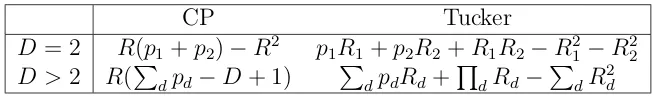
it provides a base for data adaptive selection of appropriate orders in a Tucker model. First we quickly review the number of free parameters pC for a CP model B = JB1, . . . ,BdK, with Bd∈IRpd×R. ForD= 2, pC =R(p1+p2)−R2, and for D >2, pC =
R(PD
d=1pd−D+ 1). ForD= 2, the term−R2 adjusts for the nonsingular transformation
indeterminancy for model indenfiability; for D >2, the termR(−D+ 1) adjusts for the scaling indeterminancy in the CP decomposition. See Zhou et al. (2013) for more details. Following similar arguments, we obtain that the number of free parameterspTin a Tucker model B =JG;B1, . . . ,BdK, with G∈IRR1×···×Rd and Bd∈IRpd×Rd, is
pT =
D
X
d=1
pdRd+ D
Y
d=1
Rd− D
X
d=1
R2d,
for any D. Here the term -PD
d=1R 2
d adjusts for the non-singular transformation
indeter-minancy in the Tucker decomposition. We summarize these results in Table 2.1.
Next we compare the two model sizes (degrees of freedom) under an additional as-sumption that R1 =· · ·=Rd=R. The difference becomes:
pT−pC =
0 when D= 2,
R(R−1)(R−2) when D= 3,
R(R3−4R+ 3) when D= 4,
R(RD−1−DR+D−1) when D >4.
Based on this formula, when D= 2, the Tucker model is essentially the same as the CP model. When D = 3, Tucker has the same number of parameters as CP for R = 1 or
Table 2.1: Number of free parameters in Tucker and CP models.
CP Tucker
D= 2 R(p1+p2)−R2 p1R1+p2R2+R1R2−R21−R22
D >2 R(P
dpd−D+ 1)
P
dpdRd+
Q
dRd−
P
dR
2
d
R > 2. For instance, when D = 4 and R = 3, Tucker model takes 54 more parameters than the CP model. However, one should bear in mind that the above discussion assumes
R1 = · · · = Rd = R. In reality, Tucker could require less free parameters than CP, as
shown in the illustrative example given in Section 1, since Tucker is more flexible and allows different orderRd along each dimension.
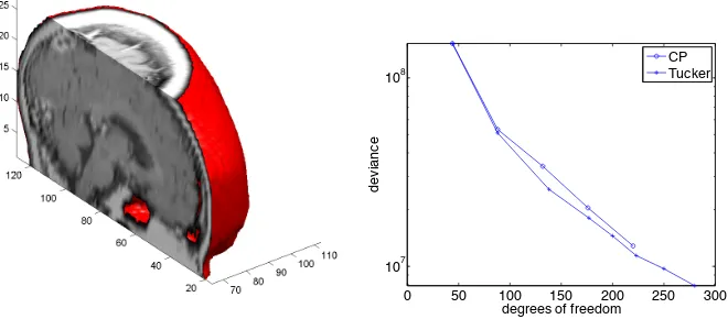
Figure 2.1 shows an example withD= 3 dimensional array covariates. Half of the true signal (brain activity map) B is displayed in the left panel, which is by no means a low rank signal. Suppose 3D images Xi are taken on n= 1,000 subjects. We simulate image
traitsXi from independent standard normals and quantitative traitsYifrom independent
normals with mean hXi,Bi and unit variance. Given the limited sample size, the hope
is to infer a reasonable low rank approximation to the activity map from the 3D image covariates. The right panel displays the model deviance versus the degrees of freedom of a series of CP and Tucker model estimates. The CP model is estimated at ranks
R = 1, . . . ,5. The Tucker model is fitted at orders (R1, R2, R3) = (1,1,1), (2,2,2), (3,3,3), (4,4,3), (4,4,4), (5,4,4), (5,5,4), and (5,5,5). We see from the plot that, under the same number of free parameters, the Tucker model could generally achieve a better model fit with a smaller deviance. (Note that the deviance is in the log scale, so a small discrepancy between the two lines translates to a large value of difference in deviance.)
0 50 100 150 200 250 300 107
108
degrees of freedom
deviance
CP Tucker
Figure 2.1: Left: half of the true signal array B. Right: Deviances of CP regression estimates at R = 1, . . . ,5, and Tucker regression estimates at orders (R1, R2, R3) = (1,1,1), (2,2,2), (3,3,3), (4,4,3), (4,4,4), (5,4,4), (5,5,4), and (5,5,5). The sample size is n= 1000.
selection problem, and we can employ a typical model selection criterion, e.g., Bayesian information criterion (BIC). It is of the form: −2 log` + log(n)pe, where ` is the
log-likelihood, and pe = pT is the effective number of parameters of the Tucker model as given in Table 2.1. We will illustrate this BIC criterion in the numerical Section 2.8.1, and will discuss some heuristic guidelines of selecting orders in Section 2.8.5.
2.5
Estimation
We pursue the maximum likelihood estimation (MLE) for the Tucker tensor regression model and develop a scalable estimation algorithm in this section. The key observation is that, although the systematic part (2.4) is not linear in G and Bd jointly, it is linear
each factor matrix Bd and the core tensor Galternately.
The algorithm consists of two core steps. First, when updating Bd ∈ IRpd×Rd with
the restBd0’s and G fixed , we rewrite the array inner product in (2.4) as
hB,Xi = hB(d),X(d)i
= hBdG(d)(BD⊗ · · · ⊗Bd+1⊗Bd−1⊗ · · · ⊗B1)T,X(d)i = hBd,X(d)(BD⊗ · · · ⊗Bd+1⊗Bd−1⊗ · · · ⊗B1)GT(d)i.
Then the problem turns into a GLM regression with Bd as the “parameter” and the
term X(d)(BD ⊗ · · · ⊗Bd+1 ⊗ Bd−1 ⊗ · · · ⊗B1)GT(d) as the “predictor”. It is a low dimensional GLM with only pdRd parameters and thus is easy to solve. Second, when
updating G∈IRR1×···×RD with all B
d’s fixed,
hB,Xi = hvec(B),vec(X)i
= h(BD⊗ · · · ⊗B1)vec(G),vec(X)i = hvec(G),(BD⊗ · · · ⊗B1)Tvec(X)i.
This implies a GLM regression with vec(G) as the “parameter” and the term (BD⊗ · · · ⊗ B1)Tvec(X) as the ”predictor”. Again this is a low dimensional regression problem with
Q
dRd parameters. For completeness, we summarize the above alternating estimation
procedure in Algorithm 1. The orthogonality between the columns of factor matrices
Bd is not enforced as in unsupervised HOSVD (Kilmer and Martin, 2004), because our
primary goal is approximating tensor signal instead of finding the principal components along each mode.
Algorithm 1 Block relaxation algorithm for fitting the Tucker tensor regression. Initialize: γ(0) = argmax
γ`(γ,0, . . . ,0), Bd(0) ∈ IR
pd×Rd a random matrix for d =
1, . . . , D, and G(0)∈IRR1×···×RD a random matrix.
repeat
for d = 1, . . . , D do
Bd(t+1) = argmaxB
d`(γ
(t),B(t+1)
1 , . . . ,B (t+1)
d−1 ,Bd,B
(t)
d+1, . . . ,B (t)
D ,G(t))
end for
G(t+1)= argmax
G`(γ(t),B
(t+1)
1 , . . . ,B (t+1)
D ,G)
γ(t+1) = argmax
γ`(γ,B1(t+1), . . . ,B (t+1)
D ,G(t+1))
until`(θ(t+1))−`(θ(t))<
relaxation algorithm monotonically increases the objective value, the stopping criterion is well-defined and the convergence properties of iterates follow from the standard theory for monotone algorithms (de Leeuw, 1994; Lange, 2010). The proof of next result is given in the Appendix.
Proposition 1. Assume (i) the log-likelihood function ` is continuous, coercive, i.e., the set {θ : `(θ) ≥ `(θ(0))} is compact, and bounded above, (ii) the objective function in each block update of Algorithm 1 is strictly concave, and (iii) the set of stationary
points (modulo nonsingular transformation indeterminancy) of `(γ,G,B1, . . . ,BD) are
isolated. We have the following results.
1. (Global Convergence) The sequence θ(t) = (γ(t),G(t),B(t)
1 , . . . ,B (t)
D ) generated by
Algorithm 1 converges to a stationary point of `(γ,G,B1, . . . ,BD).
2. (Local Convergence) Letθ(∞) = (γ(∞),G(∞),B1(∞), . . . ,BD(∞))be a strict local max-imum of `. The iterates generated by Algorithm 1 are locally attracted to θ(∞) for
2.6
Statistical Theory
In this section we study the usual large n asymptotics of the proposed Tucker tensor regression. Regularization is treated in the next section for the small or moderatencases. For simplicity, we drop the classical covariate Z in this section, but all the results can be straightforwardly extended to include Z. We also remark that, although the usually limited sample size of neuroimging studies makes the largenasymptotics seem irrelevant, we still believe such an asymptotic investigation important, for several reasons. First, when the sample size n is considerably larger than the effective number of parameters
pT, the asymptotic study tells us that the model is consistently estimating the best Tucker structure approximation to the full array model in the sense of Kullback-Liebler distance. Second, the explicit formula for score and information are not only useful for asymptotic theory but also for computation, while the identifiability issue has to be properly dealt with for the given model. Finally, the regular asymptotics can be of practical relevance, for instance, can be useful in a likelihood ratio type test in a replication study.
2.6.1
Score and Information
We first derive the score and information for the tensor regression model, which are es-sential for statistical estimation and inference. The following standard calculus notations are used. For a scalar function f,∇f is the (column) gradient vector, df = [∇f]T is the
differential, and d2f is the Hessian matrix. For a multivariate function g : IRp 7→ IRq, Dg ∈ IRp×q denotes the Jacobian matrix holding partial derivatives ∂gj
∂xi. We start from
Lemma 3. 1. The gradient ∇η(B1, . . . ,BD)∈IR Q
dRd+PDd=1pdRd is
∇η(G,B1, . . . ,BD) = [BD⊗ · · · ⊗B1 J1 J2 · · · JD]Tvec(X),
where Jd∈IR QD
d=1pd×pdRd is the Jacobian
Jd=DB(Bd) = Πd{[(BD⊗ · · · ⊗Bd+1⊗Bd−1⊗ · · · ⊗B1)GT(d)]⊗Ipd} (2.5)
and Πd is the (QDd=1pd)-by-(QDd=1pd) permutation matrix that reorders vec(B(d)) to obtain vec(B), i.e., vec(B) =Πdvec(B(d)).
2. Let the Hessian d2η(G,B
1, . . . ,BD) ∈ IR( Q
dRd+PdpdRd)×(QdRd+PdpdRd) be
parti-tioned into four blocks HG,G ∈ IR
Q
dRd×QdRd, H
G,B = HBT,G ∈ IR
Q
dRd×PdpdRd
and HB,B ∈IR
P
dpdRd×
P
dpdRd. Then H
G,G =0, HG,B has entries
h(r1,...,rD),(id,sd) = 1{rd=sd}
X
jd=id
xj1,...,jD
Y
d06=d
β(rd0) jd0 ,
and HB,B has entries
h(id,rd),(id0,rd0)= 1{d6=d0}
X
jd=id,jd0=id0
xj1,...,jD
X
sd=rd,sd0=rd0
gs1,...,sD
Y
d006=d,d0
β(sd00) jd00 .
Furthermore, HB,B can be partitioned in D2 sub-blocks as
0 ∗ ∗ ∗
H21 0 ∗ ∗
..
. ... . .. ∗
HD1 HD2 · · · 0
The elements of sub-block Hdd0 ∈IRpdRd×pd0Rd0 can be retrieved from the matrix
X(dd0)(BD ⊗ · · · ⊗Bd+1⊗Bd−1⊗ · · · ⊗Bd0+1⊗Bd0−1⊗ · · · ⊗B1)GT
(dd0).
HG,B can be partitioned into D sub-blocks as (H1, . . . ,HD). The sub-block Hd ∈
IRQdRd×pdRd has at most p
dQdRd nonzero entries which can be retrieved from the
matrix
X(d)(BD ⊗ · · · ⊗Bd+1⊗Bd−1⊗ · · · ⊗B1).
Let `(B1, . . . ,BD|y,x) = lnp(y|x,B1, . . . ,BD) be the log-density of GLM. Next
result derives the score function, Hessian, and Fisher information of the Tucker tensor regression model.
Proposition 2. Consider the tensor regression model defined by (2.3) and (2.4).
1. The score function (or score vector) is
∇`(G,B1, . . . ,BD) =
(y−µ)µ0(η)
σ2 ∇η(G,B1, . . . ,BD) (2.6)
with ∇η(G,B1, . . . ,BD) given in Lemma 3.
2. The Hessian of the log-density ` is
H(G,B1, . . . ,BD)
= −
[µ0(η)]2
σ2 −
(y−µ)θ00(η)
σ2
∇η(G,B1, . . . ,BD)dη(G,B1, . . . ,BD)
+(y−µ)θ 0(η)
σ2 d
2η(G,B
with d2η defined in Lemma 3.
3. The Fisher information matrix is
I(G,B1, . . . ,BD)
= E[−H(G,B1, . . . ,BD)]
= Var[∇`(G,B1, . . . ,BD)d`(G,B1, . . . ,BD)]
= [µ 0(η)]2
σ2 [BD⊗ · · · ⊗B1 J1. . .JD]
T
vec(X)vec(X)T
[BD⊗ · · · ⊗B1 J1. . .JD].
(2.8)
Remark: For canonical link, θ =η,θ0(η) = 1, θ00(η) = 0, and the second term of Hessian vanishes. For the classical GLM with linear systematic part (D= 1),d2η(G,B
1, . . . ,BD)
is zero and thus the third term of Hessian vanishes. For the classical GLM (D= 1) with canonical link, both second and third terms of the Hessian vanish and thus the Hessian is non-stochastic, coinciding with the information matrix.
2.6.2
Identifiability
The Tucker decomposition (2.2) is unidentifiable due to the nonsingular transformation indeterminancy. That is
JG;B1, . . . ,BDK=JG×1O1−1 × · · · ×D O−1D ;B1O1, . . . ,BDODK
for any nonsingular matricesOd ∈IRRd×Rd. This implies that the number of free
param-eters for a Tucker model is P
dpdRd+
Q
dRd−
P
dR
2
d, with the last term adjusting for
the equivalency classes.
For asymptotic consistency and normality, it is necessary to adopt a specific con-strained parameterization. It is common to impose the orthonormality constraint on the factor matrices BT
dBd = IRd, d = 1, . . . , D. However the resulting parameter space is a
manifold and much harder to deal with. We adopt an alternative parameterization that fixes the entries of the firstRd rows of Bd to be ones
B ={JG;B1, . . . ,BDK :β
(r)
id = 1, id = 1, . . . , Rd, d= 1, . . . , D}.
The formulae for score, Hessian and information in Proposition 2 require changes accord-ingly. The entries in the first Rd rows of Bd are fixed at ones and their corresponding
entries, rows and columns in score, Hessian and information need to be deleted. Choice of the restricted space B is obviously arbitrary, and excludes arrays with any entries in the first rows ofBd equal to zeros. However the set of such exceptional arrays has Lebesgue
measure zero. In specific applications, subject knowledge may suggest alternative restric-tions on the parameters.
Given a finite sample size, conditions for global identifiability of parameters are in general hard to obtain except in the linear case (D = 1). Local identifiability es-sentially requires linear independence between the “collapsed” vectors: [BD ⊗ · · · ⊗ B1 J1. . .JD]Tvec(xi)∈IR
P
dpdRd+QdRd−PdRd2.
Proposition 3 (Identifiability). Given iid data points {(yi,xi), i = 1, . . . , n} from the
B0 is locally identifiable if and only if
I(B0) =[BD ⊗ · · · ⊗B1 J1. . .JD]T
" n X
i=1
µ0(ηi)2 σ2
i
vec(xi)vec(xi)T
#
·
[BD ⊗ · · · ⊗B1 J1. . .JD]
is nonsingular.
2.6.3
Asymptotics
The asymptotics for tensor regression follow from those for MLE or M-estimation. The key observation is that the nonlinear part of tensor model (2.4) is a degree-D polyno-mial of parameters and the collection of polynopolyno-mials {hB,Xi,B ∈ B} form a
Vapnik-˘
Cervonenkis (VC) class. Then the classical uniform convergence theory applies (van der Vaart, 1998). For asymptotic normality, we need to establish that the log-likelihood func-tion of tensor regression model is quadratic mean differentiable (Lehmann and Romano, 2005). A sketch of the proof is given in the Appendix.
Theorem 1. Assume B0 ∈ B is (globally) identifiable up to permutation and the array covariates Xi are iid from a bounded underlying distribution.
1. (Consistency) The MLE is consistent, i.e., Bˆn converges to B0 in probability, in following models. (1) Normal tensor regression with a compact parameter space
B0 ⊂ B. (2) Binary tensor regression. (3) Poisson tensor regression with a compact parameter space B0 ⊂ B.
2. (Asymptotic Normality) For an interior point B0 ∈ B with nonsingular informa-tion matrix I(B0)(2.8) and Bˆn is consistent,
√
In practice it is rare that the true regression coefficient Btrue∈IRp1×···×pD is exactly a low rank tensor. However the MLE of the rank-Rtensor model converges to the maximizer of function M(B) =PBtruelnpB or equivalently PBtrueln(pB/pBtrue). In other words, the
MLE consistently estimates the best approximation (among models inB) of Btrue in the sense of Kullback-Leibler distance.
2.7
Regularized Estimation
Regularization plays a crucial role in neuroimaging analysis for several reasons. First, even after substantial dimension reduction by imposing a Tucker structure, the number of parameterspT can still exceed the number of observations n. Second, even whenn > pT, regularization could potentially be useful for stabilizing the estimates and improving the risk property. Finally, regularization is an effective way to incorporate prior scientific knowledge about brain structures. For instance, it may sometimes be reasonable to impose symmetry on the parameters along the coronal plane for MRI images.
In our context of Tucker regularized regression, there are two possible types of regular-izations, one on the core tensor Gonly, and the other on both GandBdsimultaneously.
Which regularization to use depends on the practical purpose of a scientific study. In this section, we illustrate the regularization on the core tensor, which simultaneously achieves sparsity in the number of outer products in Tucker decomposition (2.2) and shrinkage. Toward that purpose, we propose to maximize the regularized log-likelihood
`(γ,G,B1, . . . ,BD)−
X
r1,...,rD
Pη(|gr1,...,rD|, λ),
η is an index for the penalty family. Note that the penalty term above only involves elements of the core tensor, and thus regularization on G only. This formulation in-cludes a large class of penalty functions, including power family (Frank and Friedman, 1993), where Pη(|x|, λ) = λ|x|η, η ∈ (0,2], and in particular lasso (Tibshirani, 1996)
(η = 1) and ridge (η = 2); elastic net (Zou and Hastie, 2005), where Pη(|x|, λ) = λ[(η−1)x2/2 + (2−η)|x|],η ∈[1,2]; SCAD (Fan and Li, 2001), where ∂/∂|x|Pη(|x|, λ) = λ1{|x|≤λ}+ (ηλ− |x|)+/(η−1)λ1{|x|>λ} , η > 2; and MC+ penalty (Zhang, 2010), where Pη(|x|, λ) = {λ|x| −x2/(2η)}1{|x|<ηλ}+ 0.5λ2η1{|x|≥ηλ}, among many others.
Two aspects of the proposed regularized Tucker regression, parameter estimation and tuning, deserve some discussion. For regularized estimation, it incurs only slight changes in Algorithm 1. That is, when updating G, we simply fit a penalized GLM regression problem,
G(t+1) = argmaxG`(γ(t),B1(t+1), . . . ,BD(t+1),G)− X
r1,...,rD
Pη(|gr1,...,rD|, λ),
for which many software packages exist. Our implementation utilizes an efficientMatlab
toolbox for sparse regression (Zhou et al., 2011). Other steps of Algorithm 1 remain unchanged. For the regularization to remain legitimate, we constrain the column norms ofBdto be one when updating factor matricesBd. For parameter tuning, one can either
2.8
Numerical Study
We have carried out intensive numerical experiments to study the finite sample perfor-mance of the Tucker regression. Our simulations focus on four aspects: first, we demon-strate the capacity of the Tucker regression in identifying various shapes of signals; second, we compare the performance of the regularized Tucker regression with other standard sta-tistical learning techniques on vectorized images; third, we study the consistency property of the method by gradually increasing the sample size; fourth, we compare the perfor-mance of the Tucker regression with the CP regression of Zhou et al. (2013). We also examine a real MRI imaging data to illustrate the Tucker downsizing and to further compare the two tensor models.
2.8.1
Identification of Various Shapes of Signals
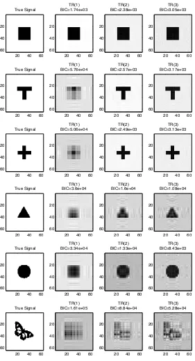
In our first example, we demonstrate that the proposed Tucker regression model, though with substantial reduction in dimension, can manage to identify a range of two dimen-sional signal shapes with varying ranks. In Figure 2.2, we list the 2D signalsB ∈IR64×64 in the first row, along with the estimates by Tucker tensor models in the second to fourth rows with orders (1,1),(2,2) and (3,3), respectively. Note that, since the orders along both dimensions are made equal, the Tucker model is to perform essentially the same as a CP model in this example, and the results are presented here for completeness. We will examine differences of the two models in later examples. The regular covariate vector
Z ∈ IR5 and image covariate X ∈ IR64×64 are randomly generated with all elements
being independent standard normals. The response Y is generated from a normal model with mean µ = γT
zero. Note that this problem differs from the usual edge detection or object recognition in imaging processing (Qiu, 2005, 2007). In our setup, all elements of the image X fol-low the same distribution. The signal region is defined through the coefficient matrix B
and needs to be inferred from the relation between Y and X after adjusting for Z. It is clear to see in Figure 2.2 that, the Tucker model yields a sound recovery of the true signals, even for those of high rank or natural shape, e.g., “disk” and “butterfly”. We also illustrate in the plot the BIC criterion in Section 2.4.4.
2.8.2
Comparison of the Regularized Tucker and Standard
Sta-tistical Models
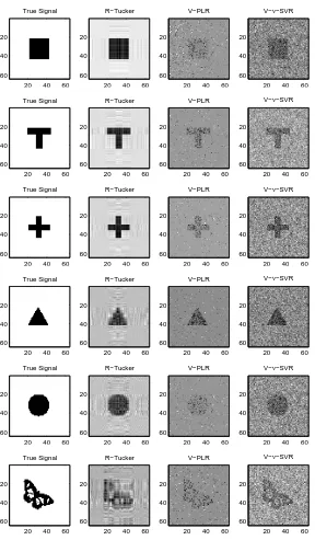
In our second example, we demonstrate the comparison of regularized Tucker model with LASSO penalty (R-Tucker), vectorized ν-SVM regression model (V-ν-SVM) and vec-torized regularized linear regression model with LASSO penalty (V-GLM). The regular covariate vectorZ ∈IR5 and image covariate X ∈IR64×64 are randomly generated with all elements being independent standard normals. The response Y is generated from a normal model with mean µ = γT
True Signal
20 40 60 20
40
60
TR(1) BIC=1.74e+03
20 40 60 20
40
60
TR(2) BIC=2.38e+03
20 40 60 20
40
60
TR(3) BIC=3.05e+03
20 40 60 20
40
60
True Signal
20 40 60 20
40
60
TR(1) BIC=5.76e+04
20 40 60 20
40
60
TR(2) BIC=2.57e+03
20 40 60 20
40
60
TR(3) BIC=3.17e+03
20 40 60 20
40
60
True Signal
20 40 60 20
40
60
TR(1) BIC=5.06e+04
20 40 60 20
40
60
TR(2) BIC=2.49e+03
20 40 60 20
40
60
TR(3) BIC=3.13e+03
20 40 60 20
40
60
True Signal
20 40 60 20
40
60
TR(1) BIC=3.6e+04
20 40 60 20
40
60
TR(2) BIC=1.6e+04
20 40 60 20
40
60
TR(3) BIC=1.08e+04
20 40 60 20
40
60
True Signal
20 40 60 20
40
60
TR(1) BIC=3.34e+04
20 40 60 20
40
60
TR(2) BIC=1.33e+04
20 40 60 20
40
60
TR(3) BIC=8.43e+03
20 40 60 20
40
60
True Signal
20 40 60 20
40
60
TR(1) BIC=1.61e+05
20 40 60 20
40
60
TR(2) BIC=8.84e+04
20 40 60 20
40
60
TR(3) BIC=5.28e+04
20 40 60 20
40
60
of the true signals.
Table 2.2: Comparison of regularized Tucker model with LASSO penalty (R-Tucker), vectorized ν-SVM regression model (V-ν-SVM) and vectorized regularized linear regres-sion model with LASSO penalty (V-GLM) in terms of root mean squared error (RMSE) of B Estimate. Results are averaged over 100 replications. Numbers in parentheses are standard errors
Rectangular ‘T’ Shape Cross Triangle Disk Butterfly R-Tucker 0.041(0.003) 0.049(0.003) 0.046(0.003) 0.108(0.005) 0.121(0.008) 0.223(0.009) V-ν-SVM 0.299(0.002) 0.233(0.001) 0.215(0.001) 0.207(0.001) 0.280(0.002) 0.284(0.002) V-GLM 0.313(0.005) 0.210(0.006) 0.179(0.006) 0.162(0.008) 0.285(0.006) 0.290(0.005)
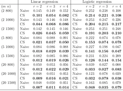
2.8.3
Performance with Increasing Sample Size
In our third example, we continue to employ a similar model as in Figure 2.2 but with a three dimensional image covariate. The dimension of X is set as p1 ×p2 ×p3, with
True Signal
20 40 60 20
40
60
R−Tucker
20 40 60 20
40
60
V−PLR
20 40 60 20
40
60
V−ν−SVR
20 40 60 20
40
60
True Signal
20 40 60 20
40
60
R−Tucker
20 40 60 20
40
60
V−PLR
20 40 60 20
40
60
V−ν−SVR
20 40 60 20
40
60
True Signal
20 40 60 20
40
60
R−Tucker
20 40 60 20
40
60
V−PLR
20 40 60 20
40
60
V−ν−SVR
20 40 60 20
40
60
True Signal
20 40 60 20
40
60
R−Tucker
20 40 60 20
40
60
V−PLR
20 40 60 20
40
60
V−ν−SVR
20 40 60 20
40
60
True Signal
20 40 60 20
40
60
R−Tucker
20 40 60 20
40
60
V−PLR
20 40 60 20
40
60
V−ν−SVR
20 40 60 20
40
60
True Signal
20 40 60 20
40
60
R−Tucker
20 40 60 20
40
60
V−PLR
20 40 60 20
40
60
V−ν−SVR
20 40 60 20
40
60
accuracy. This is not surprising though, considering the number of parameters of the model and that regularization is not employed here. The proposed tensor regression approach has been primarily designed for imaging studies with a reasonably large number of subjects. Recently, a number of such large-scale brain imaging studies are emerging. For instance, the Attention Deficit Hyperactivity Disorder Sample Initiative (ADHD, 2013) consists of over 900 participants and the Alzheimer’s Disease Neuroimaging Initiative (ADNI, 2013) database accumulates over 3,000 participants. In addition, regularization discussed in Section 2.7 and the Tucker downsizing in Section 2.4.3 can both help improve estimation given a limited sample size.
2.8.4
Comparison of the Tucker and CP Models
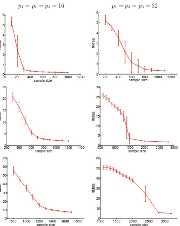
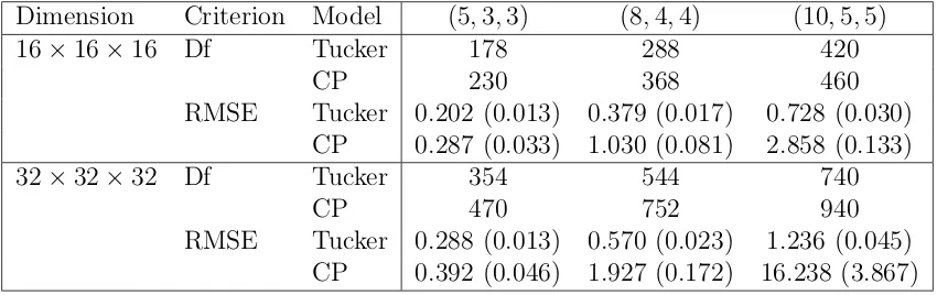
In our fourth example, we focus on comparison between the Tucker tensor model with the CP tensor model of Zhou et al. (2013). We generate a normal response, and the 3D signal array B with dimensions p1, p2, p3 and the d-ranks r1, r2, r3. Here, the d-rank is defined as the column rank of the mode-d matricization B(d) of B. We set p1 = p2 = p3 = 16 and 32, and (r1, r2, r3) = (5,3,3),(8,4,4) and (10,5,5), respectively. The sample size is 2000. We fit a Tucker model withRd =rd, and a CP model with R = maxrd,d= 1,2,3.
p1 =p2 =p3 = 16 p1 =p2 =p3 = 32
0 200 400 600 800 1000 1200
0 1 2 3 4 5 6 sample size RMSE
200 400 600 800 1000 1200
0 1 2 3 4 5 6 sample size RMSE
2000 400 600 800 1000 1200 1400 5 10 15 20 25 sample size RMSE
5000 1000 1500 2000 2500 3000 5 10 15 20 25 30 sample size RMSE
800 1000 1200 1400 1600 1800 0 10 20 30 40 50 60 70 sample size RMSE
10000 1500 2000 2500 3000
10 20 30 40 50 60 sample size RMSE
Figure 2.4: Root mean squared error (RMSE) of the tensor parameter estimate versus the sample size. Reported are the average and standard deviation of RMSE based on 100 data replications. Top: R1 = R2 = R3 = 2; Middle: R1 = R2 = R3 = 5; Bottome:
Table 2.3: Comparison of the Tucker and CP models. Reported are the average and standard deviation (in the parenthesis) of the root mean squared error, all based on 100 data replications.
Dimension Criterion Model (5,3,3) (8,4,4) (10,5,5)
16×16×16 Df Tucker 178 288 420
CP 230 368 460
RMSE Tucker 0.202 (0.013) 0.379 (0.017) 0.728 (0.030) CP 0.287 (0.033) 1.030 (0.081) 2.858 (0.133)
32×32×32 Df Tucker 354 544 740
CP 470 752 940
RMSE Tucker 0.288 (0.013) 0.570 (0.023) 1.236 (0.045) CP 0.392 (0.046) 1.927 (0.172) 16.238 (3.867)
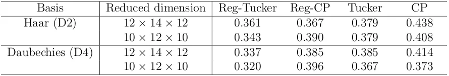
Burner data, http://neurobureau.projects.nitrc.org/ADHD200/Data.html). In addition to the MRI image predictor, we also include the subjects’ age, gender and handiness as regular covariates. The response is the binary diagnosis status.
The original image size wasp1×p2×p3 = 121×145×121. We employ the Tucker down-sizing in Section 2.4.3. More specifically, we first choose a wavelet basis forBd∈IRpdטpd,
then transform the image predictor fromX to ˜X =JX;BT
1, . . . ,BDTK. We pre-specify the
values of ˜pd’s that are about tenth of the original dimensionspd, and equivalently, we fit
a Tucker tensor regression with the image predictor dimension downsized to ˜p1×p˜2×p˜3. In our example, we have experimented with a set of values of ˜pd’s, and the results are
qualitatively similar. We report two sets, ˜p1 = 12, ˜p2 = 14, ˜p3 = 12, and ˜p1 = 10, ˜p2 = 12, ˜
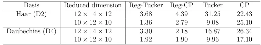
p3 = 10. We have also experimented with the Haar wavelet basis (Daubechies D2) and the Daubechies D4 wavelet basis, which again show similar qualitative patterns.
For ˜p1 = 12,p˜2 = 14,p˜3 = 12, we fit a Tucker tensor model with R1 =R2 =R3 = 3, resulting in 114 free parameters, and fit a CP tensor model with R = 4, resulting in 144 free parameters. For ˜p1 = 10,p˜2 = 12,p˜3 = 10, we fit a Tucker tensor model with
R1 = R2 = 2 and R3 = 3, resulting in 71 free parameters, and fit a CP tensor model with R = 4, resulting in 120 free parameters. We have chosen those orders based on the following considerations. First, the number of free parameters of the Tucker and CP models are comparable. Second, at each step of GLM model fit, we ensure that the ratio between the sample size n and the number of parameters under estimation in that step ˜
pd×Rd satisfies a heuristic rule of greater than two in normal models and greater than
five in logistic models. In the Tucker model, we also ensure the ratio between n and the number of parameters in the core tensor estimation Q
dRd satisfies this rule. We note
Table 2.4: ADHD testing data misclassification error.
Basis Reduced dimension Reg-Tucker Reg-CP Tucker CP
Haar (D2) 12×14×12 0.361 0.367 0.379 0.438
10×12×10 0.343 0.390 0.379 0.408
Daubechies (D4) 12×14×12 0.337 0.385 0.385 0.414
10×12×10 0.320 0.396 0.367 0.373
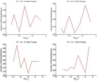
CP model with the same orders, while the penalty parameter is tuned based on 5-fold cross validation of the training data. Figure 2.5 shows that we select λ with the smallest number of misclassifications in regularized Tucker model.
We evaluate each model by comparing the misclassification error rate on the inde-pendent testing set. The results are shown in Table 2.4. We see from the table that, the regularized Tucker model performs the best, which echoes the findings in our simulations above. We also remark that, considering the fact that the ratio of case-control is about 4:5 in the testing data, the misclassification rate from 0.32 to 0.36 achieved by the regularized Tucker model indicates a fairly sound classification accuracy. On the other hand, we note that, a key advantage of our proposed approach is its capability of suggesting a useful model rather than the classification accuracy per se. This is different from black-box type machine learning based imaging classifiers.
−15 −10 −5 0 260
270 280 290 300 310
10 × 12 × 10 Haar Tuning
log10 λ
Number of Misclassifications
−15 −10 −5 0 270
275 280 285 290
10 × 12 × 10 D4 Tuning
log10λ
Number of Misclassifications
−16 −14 −12 −10 −8 −6 265
270 275 280 285 290 295 300 305
12 × 14 × 12 Haar Tuning
log10λ
Number of Misclassifications
−16 −14 −12 −10 −8 −6 270
280 290 300 310 320 330
12 × 14 × 12 D4 Tuning
log10λ
Number of Misclassifications
Figure 2.5: Grid search for regularization parameter,λ, in regularized Tucker model. λ
Table 2.5: ADHD model fitting run time (in seconds).
Basis Reduced dimension Reg-Tucker Reg-CP Tucker CP
Haar (D2) 12×14×12 3.68 4.39 31.25 22.43
10×12×10 1.36 2.79 9.08 25.10
Daubechies (D4) 12×14×12 3.30 2.18 16.87 26.34
10×12×10 1.92 1.90 9.96 17.10
2.9
Discussion
2.9.1
Summary
We have proposed a tensor regression model based on the Tucker decomposition. In-cluding the CP tensor regression (Zhou et al., 2013) as a special case, Tucker model provides a more flexible framework for regression with imaging covariates. We develop a fast estimation algorithm, a general regularization procedure, and the associated asymp-totic properties. In addition, we provide a detailed comparison, both analytically and numerically, of the Tucker and CP tensor models.
In real imaging analysis, the signal hardly has an exact low rank. On the other hand, given the limited sample size, a low rank estimate often provides a reasonable approxi-mation to the true signal. This is why the low rank models such as the Tucker and CP could offer a sound recovery of even a complex signal.
Table 2.6: Fitting run time for recovering ‘triangle’ shape (in seconds) at rank 1, 2, 3 and 4. Reported are the median time of 100 runs.
r= 1 r = 2 r = 3 r= 4 Triangle 0.30 1.21 4.22 9.62
Table 2.7: Computing time comparison of the Tucker and CP models in Section 2.8.4. Reported are median time (in seconds) over 100 runs.
Dimension Model (5,3,3) (8,4,4) (10,5,5) 16×16×16 Tucker 1.03 1.71 3.03
CP 7.47 11.51 15.64
32×32×32 Tucker 9.93 21.51 50.52
CP 28.36 59.82 89.81
2.9.2
Computation Time
We conduct a numerical experiment to study the computing time of proposed Tucker model. We adopt the setting in Section 2.8.1 and use the ‘triangle’ shape. We test the computing time by running the algorithm on one data set from 100 random starting points. Table 2.6 displays the median wall clock run times.
In addition, we compare the computing time for Tucker and CP under the simulation setup in Section 2.8.4. We test the computing time by running the algorithms on one data set from 100 random starting points. Table 2.7 displays the results.
strategy given in Section 2.7.
All run times were recorded on a standard laptop computer with a 3.4 GHz Intel i7 CPU.