Sparse Linear Discriminant Analysis with
Applications to High Dimensional Low Sample
Size Data
Zhihua Qiao,
∗Lan Zhou
†and Jianhua Z. Huang
‡Abstract— This paper develops a method for auto-matically incorporating variable selection in Fisher’s linear discriminant analysis (LDA). Utilizing the con-nection of Fisher’s LDA and a generalized eigenvalue problem, our approach applies the method of regu-larization to obtain sparse linear discriminant tors, where “sparse” means that the discriminant vec-tors have only a small number of nonzero compo-nents. Our sparse LDA procedure is especially effec-tive in the so-called high dimensional, low sample size (HDLSS) settings, where LDA possesses the “data piling” property, that is, it maps all points from the same class in the training data to a common point, and so when viewed along the LDA projection direc-tions, the data are piled up. Data piling indicates overfitting and usually results in poor out-of-sample classification. By incorporating variable selection, the sparse LDA overcomes the data piling problem. The underlying assumption is that, among the large num-ber of variables there are many irrelevant or redun-dant variables for the purpose of classification. By using only important or significant variables we es-sentially deal with a lower dimensional problem. Both synthetic and real data sets are used to illustrate the proposed method.
Keywords: Classification, linear discriminant analysis, variable selection, regularization, sparse LDA
1
Introduction
Fisher’s linear discriminant analysis (LDA) is typically used as a feature extraction or dimension reduction step before classification. The most popular tool for di-mensionality reduction is principal components analysis (PCA, Pearson 1901, Hotelling 1933). PCA searches for a few directions to project the data such that the pro-jected data explain most of the variability in the original
∗MIT Sloan School of Management, 50 Memorial Drive,
E52-456, Cambridge, MA 02142, USA. Email: [email protected]
†Department of Statistics, Texas A&M University, 447
Blocker Building, College Station, TX 77843-3143, USA. Email: [email protected].
‡Corresponding Author. Department of Statistics, Texas A&M
University, 447 Blocker Building, College Station, TX 77843-3143, USA. Email:[email protected].
data. In this way, one obtains a low dimensional repre-sentation of the data without losing much information. Such attempt to reduce dimensionality can be described as “parsimonious summarization” of the data. However, since PCA targets for the unsupervised problem, it would not be suitable for classification problems.
For a classification problem, how does one utilize the class information in finding informative projections of the data? Fisher (1936) proposed a classic approach: Find the projection direction such that for the projected data, the between-class variance is maximized relative to the within-class variance. Additional projection directions with decreasing importance in discrimination can be de-fined in sequence. The total number of projection di-rections one can define is one less than the number of classes. Once the projection directions are identified, the data can be projected to these directions to obtain the reduced data, which are usually called discriminant vari-ables. For the discriminant variables, any classification method can be carried out, such as nearest centroid, k -nearest neighborhood, and support vector machines. A particular advantage of Fisher’s idea is that one can ex-ploit the graphical tools. For example, with two projec-tion direcprojec-tions one can view the data in a two-dimensional plot, color-coding the classes.
−4 −2 0 2 4
LDA training
−4 −2 0 2 4
Theoretical LDA training
−4 −2 0 2 4
LDA test
−4 −2 0 2 4
Theoretical LDA test
[image:2.612.66.273.55.237.2]Projected data
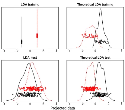
Figure 1: A simulated example with two classes. Plotted are the projected data using the estimated and theoretical LDA directions. Top panels are for training data; bot-tom panels for test data. Left panels use estimated LDA directions; right panels the theoretical directions. The in-sample and out-of-sample error rates are 0 and 32% respectively, when applying the nearest centroid method to the data projected to the estimated LDA direction. The dimension of the data is 100 and there are 25 cases for each class.
we incorporate variable selection in LDA.
We find that variable selection may provide a promising approach to deal with a very challenging case of data mining: the high dimensional, low sample size (HDLSS, Marron et al. 2007) settings. The HDLSS means that the dimension of the data vectors is larger (often much larger) than the sample size (the number of data vectors available). HDLSS data occur in many applied areas such as genetic micro-array analysis, chemometrics, medical image analysis, text classification, and face recognition. As pointed out by Marron et al., classical multivariate statistical methods often fail to give a meaningful analysis in HDLSS contexts.
Ahn and Marron (2007) and Marron et al. (2007) dis-covered an interesting phenomenon called “data piling” for discriminant analysis in HDLSS settings. Data piling means that when the data are projected onto some pro-jection direction, many of the propro-jections are exactly the same, that is, the data pile up on top of each other. Data piling is not a useful property for discrimination, because the corresponding direction vector is driven by very par-ticular aspects of the realization of the training data at hand. Data piling direction provides perfect separation of classes in sample, but it inevitably has bad generalization property.
The Fisher’s LDA is not applicable to HDLSS settings
since the within-class covariance matrix is singular. Sev-eral extensions of LDA that can overcome the singular-ity problem, including pseudo-inverse LDA, Uncorrelated LDA (Ye et al. 2006), and Orthogonal LDA (Ye 2005), all possess the data piling problem. As an illustration of the data piling problem, Figure 1 provides views of two simulated data sets, one of which serves as a training data set, shown in the first row, the other the test data set, shown in the second row. The data are projected onto some direction vector and the projections are represented as a “jitter plot”, with the horizontal coordinate repre-senting the projection, and with a random vertical coor-dinate used for visual separation of the points. A kernel density estimate is also shown in each plot to reveal the structure of the projected data. Two methods are con-sidered to find a projection direction in Figure 1. Fisher’s LDA (using pseudo-inverse of the with-in class covariance matrix) is applied to the training data set to obtain the projection direction for the left panels, while the theo-retical LDA direction, which is based on the knowledge of the true within-class and between-class covariance ma-trices, is used for the right panels. The LDA direction estimated using training data possesses obvious data pil-ing and overfittpil-ing. The perfect class separation in sam-ple does not translate to good separation out of samsam-ple. In contrast, the projections to the theoretical LDA di-rection for the two data sets have similar distributional properties.
One contribution of the present paper is to offer a method to deal with the “data piling” problem in HDLSS set-tings. If a small number of significant variables suffice for discrimination, then identifying these variables may help prevent “data piling” in the training data and con-sequently yield good out-of-sample classification. In Sec-tion 4.1, the same data sets will be projected to the sparse LDA direction estimated using the training data. We will see that these projections will resemble the distributional behavior on the right panels of Figure 1 that are based on the theoretical LDA directions. The main message is that without variable selection, LDA is subject to data piling and leads to bad out-of-sample classification; with vari-able selection, data piling on training data is prevented and thereby good classification on test data is obtained.
2
Review of Fisher’s LDA
Discriminant analysis has been a standard topic in any multivariate analysis text book (e.g., Mardia, et al., 1979). A common approach to discriminant analysis is to apply the decision theory framework. In this frame-work, one assumes a parametric form of the population distribution and a prior probability for each class, then derives the Bayesian decision rule for classification. If the assumed population distribution for each class is multi-variate normal and the covariances are common across different classes, the resulting decision rule is based on a linear function of the input data and therefore called linear discriminant analysis (LDA). Although the strong assumptions used in this derivation of LDA are not true in many applications, LDA has been proven very effective. This is mainly due to the fact that a simple, linear model is more robust against noise, and less likely to overfit.
An alternative approach to discrimination analysis can be made by merely looking for a “sensible” rule to dis-criminate the classes without assuming any particular parametric form for the distribution of the populations. Fisher’s LDA looks for the linear functionaTxsuch that
the ratio of the between-class sum of squares to the within-class sum of squares is maximized. Formally, sup-pose there arek classes and letxij, j= 1, . . . , ni,be
vec-tors of observations from thei-th class, i= 1, . . . , k. Set n=n1+. . . , nk and let ¯xi denote the mean of the i-th
class. Let
Xn×p= (x11, . . . , x1n1, . . . , x T
k1, . . . , xTknk)
T
andy=Xa, then Fisher’s LDA solves
max
a
Pk
i=1ni(¯yi−y¯)2
Pk
i=1
Pni
j=1(yij−y¯i)2
, (1)
where ¯yi is the mean of thei-th sub-vectoryi ofy,
corre-sponding to thei-th class. SubstitutingybyXa, we can rewrite the within-class sum of squares as
k
X
i=1 ni
X
j=1
(yij−y¯i)2=aT k
X
i=1 ni
X
j=1
(xij−x¯i)(xij−x¯i)Ta
def
= aTΣwa,
and the between-class sum of squares as
k
X
i=1
ni(¯yi−y¯)2= k
X
i=1
ni{aT(¯xi−x¯)}2
=aT
k
X
i=1
ni(¯xi−x¯)(¯xi−x¯)Ta def
= aTΣba.
Therefore the ratio is given by
aTΣba/aTΣwa.
Ifa1is the vector that maximizes the ratio, one can find
the next direction a2 orthogonal in Σw to a1, such that
the ratio is maximized; and the additional directions can be computed in sequence similarly. The projection direc-tions ai are usually called discriminant coordinates and
the linear functionsaT
ixare called Fisher’s linear
discrim-inant functions. Fisher’s criterion is intuitively sound be-cause it is relatively easy to tell the classes apart if the between-class sum of squares for y is large relative to the within-class sum of squares. Alternatively, Fisher’s criterion can be understood as dimension reduction us-ing principal components analysis on the class centroids standardized by the common within-class covariance ma-trix.
The problem (1) was Fisher’s original formulation of LDA. Another formulation of LDA popular in the pat-tern recognition literature (i.e., Fukunaga, 1990) is to solve the optimization problem
max
A
tr (ATΣwA)−1ATΣbA (2)
subject to ATA = I. Both (1) and (2) are equivalent
to finding a’s that satisfy Σba=ηΣwa, for η 6= 0. This
is a generalized eigenvalue problem. There are no more than min(p, k−1) eigenvectors corresponding to nonzero eigenvalues, since the rank of the matrix Σb is bounded
from above by min(p, k−1).
In this paper, we view LDA as a supervised dimension reduction tool that searches for suitable projection di-rections, and therefore refer to eigenvectors ai’s as the
discriminant directions or discriminant vectors. These discriminant directions/vectors are useful for data visu-alization and also for classification. By projecting thep -dimensional data onto the q-dimensional space spanned by the first q (q ≤ min(p, k−1)) discriminant vectors, we reduce thep-dimensional data to q-dimensional data. The low dimensional data can be easily visualized, us-ing for example pairwise scatterplots. Any methods of discriminant analysis, such as nearest centroid method, nearest neighborhood method, and the support vector machines, can be applied to the reduced data to develop classification rules.
To facilitate subsequent discussion, we introduce some notations here. Definen×pmatrices
Hw=X−
en1x¯T 1
.. . enkx¯T
k
andHb=
en1(¯x1−¯x)T
.. . enk(¯x
k−x¯)T
,
whereeni is a column vector of ones with lengthn
iande
is a column vector of ones with lengthn. It is clear that with these notations, we have
Notice that the matrix Hb can be reduced to a lower
dimension (k×p) matrix
(√n1(¯x1−x¯), . . . ,√nk(¯xk−x¯))T, (3)
which also satisfies Σb =HbTHb. In the discussion that
follows, this latter form ofHbis used throughout without
further mentioning.
3
Sparse Discriminant Vectors
When Σw is positive definite, the first discriminant
di-rection vectorain Fisher’s LDA is the eigenvector corre-sponding to the largest eigenvalue of the following gener-alized eigenvalue problem
Σbβ=ηΣwβ. (4)
To incorporate variable selection in LDA corresponds to making the eigenvectorasparse. Here “sparsity” means that the eigenvectorahas only a few nonzero components or it has lots of zero components. It is not so obvious how to achieve this. However, variable selection methods are well studied for linear regression problems and those methods are useful in suggesting a feasible approach to extracting sparse eigenvectors.
LASSO (Tibshirani, 1996) is a penalized least squares method that imposes a constraint on theL1norm of
re-gression coefficients. Specifically, the LASSO solves the following optimization problem
min
β kY −Xβk 2+λ
kβk1,
where Y, X are the response vector and design matrix respectively, andβ is the vector of regression coefficients. Due to the nature of the L1 penalty, some components
of β will be shrunk to exact zero if λ is large enough. Therefore the LASSO can produce a sparse coefficient vectorβ, which makes it a variable selection method.
3.1
Link of generalized eigenvalue problems
to regressions
Our approach for obtaining sparse discriminant vectors is an extension of the sparse PCA method of Zou et al. (2006). It first relates the discriminant vector to a regression coefficient vector by transforming the general-ized eigenvalue problem to a regression-type problem, and then apply penalized least squares with an L1 penalty.
The following theorem will serve our purpose.
Theorem 1. Suppose Σw is positive definite and
de-note its Cholesky decomposition as Σw =RTwRw, where
Rw∈Rp×pis an upper triangular matrix. LetHb ∈Rk×p
be defined as in (3). Let V1, . . . , Vq (q ≤min(p, k−1))
denote the eigenvectors of problem (4) corresponding to
the q largest eigenvalues λ1 ≥ λ2 ≥ · · · ≥ λq. Let
Ap×q = [α1, . . . , αq]andBp×q = [β1, . . . , βq]. For λ >0,
letAbandBb be the solution to the following problem
min
A,B k
X
i=1
kR−wTHb,i−ABTHb,ik2+λ
q
X
j=1
βjTΣwβj,
subject to ATA=Iq×q,
(5)
where Hb,i =√ni(¯xi−x¯)T is the i-th row of Hb. Then
ˆ
βj, j = 1, . . . , q, span the same linear space as Vj, j =
1, . . . , q.
To prove Theorem 1, we need the following Lemma.
Lemma 1. Let M be a p×psymmetric positive
semi-definite matrix. Assume q < p and the eigenvalues of
M satisfy d11 ≥ · · · ≥dqq > dq+1,q+1 ≥ · · · ≥dpp ≥0.
Thep×qmatrixAthat maximizestr (ATM A)under the
constrain that ATA =I has the formA = V
1U1 where
V1 consists the first q eigenvectors of M and U1 is an
arbitrary q×q orthogonal matrix.
Proof of Lemma 1. Let the eigenvalue decomposition of
M be M = V DVT, where V is orthogonal and D = diag(d11, . . . , dpp) is diagonal, both are p×p matrices.
Note that tr (ATM A) = tr (ATV DVTA). LetU =VTA,
which is ap×qmatrix. ThenA=V U. Moreover,UTU =
ATV VTA = I, which means that U has orthonormal
columns. Denote the rows ofU byuT
1, . . . , uTp. Then
tr (ATM A) = tr (UTDU) = p
X
i=1
diitr (uiuTi ) = p
X
i=1
dii|ui|2.
Since U has orthonormal columns, |ui|2 ≤ 1 for i =
1, . . . , p and Ppi=1|ui|2 = q. The problem reduces to
maximizingPpi=1dii|ui|2subject to the constraints that
|ui|2 ≤ 1 for i = 1, . . . , p and Ppi=1|ui|2 = q. Note
that d11 ≥ · · · ≥ dqq > dq+1,q+1· · · ≥ dpp > 0 are
arranged in decreasing order. It is clear that the opti-mization problem is solved by |u1| =· · · =|uq| = 1 and
|uq+1| = · · · = |up| = 0. This implies that the first q
rows ofU form aq×qorthogonal matrix, denoted asU1,
and the rest rows of U consist of only zeros. Partition V = (V1, V2) whereV1isp×q. Then we haveA=V1U1,
which is the desired result.
Now we are ready to prove Theorem 1.
Proof of Theorem 1. Using (9) we see that the optimal
B= [β1, . . . , βq] for fixedAare
ˆ
βj= (Σb+λΣw)−1ΣbR−1αj,
or equivalently
b
Then we substitute Bb into the objective function of (5) and find that we need to maximize the object
tr{ATR−T
w Σb(Σb+λΣw)−1ΣbR−w1A} (7)
as a function of Asubject toATA=I.
Denote theqleading eigenvectors ofR−T
w ΣbR−w1 byE=
[η1, . . . , ηq] so that R−wTΣbR−w1 = EΛET where Λ is an
q×q diagonal matrix of eigenvalues. The columns ofE are also theqleading eigenvectors of the matrix
R−T
w Σb(Σb+λΣw)−1ΣbR−w1
=R−T
w ΣbR−w1(R
−T
w ΣbR−w1+λI)
−1R−T
w ΣbRw−1.
Thus, according Lemma 1, theAbthat maximizes (7) sat-isfies Ab=EP whereP is an arbitrary q×qorthogonal matrix. Substituting thisAbinto equation (6) results in
b
B=R−1
w (R
−T
w ΣbR−w1+λI)
−1R−T
w ΣbRw−1Ab
=R−1
w (EΛET +λI)
−1EΛETEP
=R−1
w E(Λ +λI)
−1ΛP
Note that the q leading eigenvectors of the generalized eigenvalue problem (4) are columns ofV =R−1
w E.
There-fore,Bb=V(Λ+λI)−1ΛP.The desired result follows.
From theorem 1, we know that ifW is positive definite, then theBβ = (β1, . . . , βq) that solves the optimization
problem (5) contains the firstqdiscriminant vectors. The optimization problem (5) can be solved by iteratively minimizing overA and B. The update ofA for fixedB is a Procrustes problem (Gower and Dijksterhuis 2004). To see this, note that
k
X
i=1
kR−T
w Hb,i−ABTHb,ik2
=kHbRw−1−HbBATk2
= tr{(HbR−w1−HbBAT)(HbR−w1−HbBAT)T}
= tr{HbR−w1R
−T
w HbT +HbBBTHbT}
−2 tr{BTHbTHbR−w1A};
(8)
we have used ATA = I to obtain the last
equal-ity. Thus, if B is fixed, the update of A maximizes tr{BTHT
b HbR−w1A}subject to the constraint thatA has
orthonormal columns. This is an inner-product version of projection Procrustes that has an analytical solution. The solution is given by computing the singular value decomposition
R−T
w (HbTHb)B =U DVT,
whereU (p×q) has orthonormal columns andV (q×q) is orthogonal, and setting Ab = U VT. (See Cliff, 1966,
Section 3 of Gower and Jijksterhuis, 2004, or Theorem 4 of Zou et al. 2006).
The update ofBfor fixedAis a regression-type problem. To see this, let A⊥ be an orthogonal matrix such that
[A;A⊥] is p×p orthogonal; this is feasible since A has
orthonormal columns. Then we have that
kHbR−w1−HbBATk2
=kHbR−w1[A;A⊥]−HbBAT[A;A⊥]k2
=kHbR−w1A−HbBk2+kHbR−w1A⊥k2
=
q
X
j=1
kHbR−w1αj−Hbβjk2+kHbR−w1A⊥k2.
IfAis fixed, then theB that optimizes (5) solves
min
B q
X
j=1
{kHbRw−1αj−Hbβjk2+λβTjΣwβj}, (9)
which is equivalent to q independent ridge regression problems.
3.2
Sparse eigenvectors
The connection to a regression-type problem of the opti-mization problem for extracting the discriminant vectors suggests an approach to produce sparse discriminant vec-tors. As in the LASSO, by adding an L1 penalty to the
objective function in the regression problem, we can ob-tain sparse regression coefficients. Therefore we consider the optimization problem
min
A,B q
X
j=1
{kHbR−w1αj−Hbβjk2
+λβjTΣwβj+λ1,jkβjk1},
(10)
subject toATA=I
q×q, wherekβjk1 is the 1-norm of the
vectorβj, or equivalently,
min
A,B k
X
i=1
kR−T
w Hb,i−ABTHb,ik2
+λ
q
X
j=1
βjΣwβj+ q
X
j=1
λ1,jkβjk1,
(11)
subject to ATA=I
q×q. Whereas the sameλis used for
all q directions, different λ1,j’s are allowed to penalize
different discriminant directions.
The optimization problem (10) or (11) can be numerically solved by alternating optimization overA andB.
• B given A: For each j, let Y∗
j = HbR−w1αj. For
prob-lems
min
βj k Y∗
j −Hbβjk2+λβjTΣwβj+λ1,jkβjk1,
j= 1, . . . , q. (12)
• A given B: For fixed B, we can ignore the penalty
term in (11) and need only minimize
k
X
i=1
kRw−THb,i−ABTHb,ik2=kHbR−w1−HbBATk2
subject toATA=I
q×q. The solution is obtained by
computing the singular value decomposition
R−T
w (HbTHb)B =U DVT
and lettingAb=U VT.
Using the Cholesky decomposition Σw =RTwRw, we see
that for eachj, (12) is equivalent to minimization of
kYej−W βf jk2+λ1,jkβjk1,
where Yej = (Yj∗T,0p×p)T and fW = (HbT, RTw)T. This is
a LASSO-type optimization problem where efficient im-plementations exist such as LARS (Efron et al. 2004).
Algorithm 1 summarizes the steps of our Sparse LDA procedure described above.
Remarks: 1. Theorem 1 implies that the solution of the optimization problem (5) is independent of the value of λ. This does not necessarily imply that the solution of the regularized problem (11) is also independent of λ. However, our empirical study suggests that the solution is very stable whenλvaries in a wide range, for example in (0.01,10000).
2. We can useK-fold cross validation (CV) to select the optimal tuning parameters{λ1,j}. We use the error rate
of a specified classification method such as the nearest centroid or nearest neighbor method applied on the pro-jected data to generate the cross validation score. Specif-ically, we randomly split the data into K parts. Fixing one part at a time as the test data, we apply the Sparse LDA to the rest of the data (treated as training data) to find the sparse discriminant vectors. Then we project all the data onto these discriminant vectors, apply a given classification method to the training data, and calculate the classification error using the test data. After we re-peat this K times, with one part as test data at a time, we combine the classification errors as the selection crite-rion. When the dimension of the input data is very large, the numerical algorithm becomes time-consuming and we can letλ1,1=· · ·=λ1,q to expedite computation.
Algorithm 1Sparse LDA Algorithm
1. Form the matricesHb∈Rk×p andHw∈Rn×p from
the data as follows
Hw=X−
en1x¯T 1
.. . enkx¯T
k
andHb=
√n
1(¯x1−x¯)
.. .
√n
k(¯xk−x¯)
.
2. Compute the upper triangular matrix Rw ∈ Rp×p
from the Cholesky decomposition of HT
wHw such
thatHT
wHw=RTwRw.
3. Solveqindependent LASSO problems
min
βj βT
j (WfTWf)βj−2˜yTfW βj+λ1kβjk1,
where
f
W(n+p)×p=
Hb
√
λRw
,y˜(n+p)×1=
HbR−w1αj
0
.
4. Compute the singular value decomposition R−T
w (HbTHb)B =U DVT and letA=U VT.
5. Repeat steps 3 and 4 until converges.
3.3
Sparse regularized LDA
When the number of variables exceeds the sample size, i.e., the high dimensional, low sample size (HDLSS) set-tings according to Marron et al. (2005), the within-class covariance matrix is singular and the method proposed above breaks down. One method to circumvent this sin-gularity problem is to regularize the within-class covari-ance, similar to the regularization method as used in ridge regression.
Consider a standard linear regression with the design ma-trixX. When X is collinear or close to being collinear, the normal equation XTXβ = XTY is ill-conditioned
and can not produce a stable solution. To stabilize the solution, ridge regression adds a positive multiple of the identity matrix to the Gram matrixXTX in forming the
normal equation, that is, (XTX+γI)β =XTY.
Simi-larly, when the within-class covariance matrix Σw is
sin-gular, we can replace it by Σw+γI when applying LDA.
Algorithm 2Sparse rLDA Algorithm
1. Form the matrixHB ∈Rk×p andHW ∈Rn×p from
the data as follows
HW =X−
en1x¯T 1
.. . enkx¯T
k
HB = (√n1(¯x1−x¯), . . . ,√nk(¯xk−x¯))T
2. Compute upper triangular matrix Rw ∈Rp×p from
the Cholesky decomposition of Σw+ (γ/p) tr (Σw)I
such that Σw+ (γ/p) tr (Σw)I=RTwRw.
3. Solveqindependent LASSO problems
min
βj
βjT(WfTfW)βj−2˜yTW βf j+λ1kβjk1, (13)
where
f
W(n+p)×p=
HB
√
λRW
,y˜(n+p)×1=
HBR−W1αj
0
.
4. Compute the singular value decomposition R−T
W (HBTHB)B=U DVT and letA=U VT.
5. Repeat steps 3 and 4 until converges.
Consider the generalized eigenvalue problem
Σbβ =η
Σw+γ
tr (Σw)
p I
β,
where γis a regularization parameter. The identity ma-trix is scaled by tr (Σw)/p so that the matrices Σw and
{tr (Σw)/p}I have the same trace. We refer to this
prob-lem as regularized LDA (rLDA for short). Following the same development as in Section 3.2, we see that the eigenvectorsβ1, . . . , βq, associated with the firstqlargest
eigenvalues of the generalized eigenvalue problem can be obtained up to a scaling constant as the solution to the following regression-type problem
min
A∈Rp×q
B∈Rp×q
k
X
i=1
kR−T
w Hb,i−ABTHb,ik2
+λ
q
X
j=1
βT j
Σw+γ
tr (Σw)
p I
βj,
subject to ATA = I
q×q, where B = [β1, . . . , βq]. This
connection suggests using theL1penalty to obtain
spar-sity for theβj’s.
We define the first q sparse discriminant directions
β1, . . . , βq as the solutions to the following optimization
problem
min
A∈Rp×q
B∈Rp×q
k
X
i=1
kR−T
w Hb,i−ABTHb,ik2
+λ
q
X
j=1
βjT
Σw+γtr (Σw)
p I
βj+ q
X
j=1
λ1,jkβjk1,
(14)
subject to ATA = I
q×q, where B = [β1, . . . , βq].
Al-gorithm 1 can be modified to obtain the sparse rLDA directions. The resulting algorithm is summarized in Al-gorithm 2. The two alAl-gorithms only differ in step 2.
Remark: In (14), γ is a tuning parameter that controls the strength of regularization of the within-class covari-ance matrix. A large value of γ will bias too much the within-class covariance matrix towards identity matrix. There are two helpful criteria for choosing γ. First, if the sample size is small and the dimension is high, then the within-class covariance matrix is not accurately es-timated and therefore we want to employ a high degree of regularization by using a relatively large value of γ. Second, we can exploit the graphical tools to choose a suitableγ with the aid of data visualization. For exam-ple, we seek aγthat yields a good separation of classes for the training data set. In our empirical studies, however, we find that the results of sparse rLDA are not sensitive to the choice ofγ if a small value that is less than 0.1 is used. We shall use γ = 0.05 for the empirical results to be presented in Sections 4 and 5. More careful studies of choice of γare left for future research.
4
Simulated Data
4.1
Two classes
Our first simulation example contains training data set of size 25 for each of the two classes and test data set of size 100 for each class. The input dataX has dimension p= 100 so this is a HDLSS setting. Only the first two variables of X can distinguish the two classes, and the remaining 98 variables are irrelevant for discrimination. The distribution of each class is
xi∼
N2(µi,Σw,2)
Np−2(0, Ip−2)
, i= 1,2,
µi=
0
±0.9
, Σw,2=
1 0.7 0.7 1
.
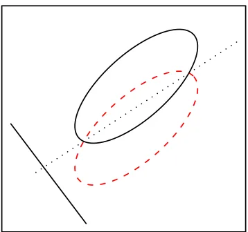
Figure 2: The theoretical projection direction and the ellipses of the population distributions of the two classes.
deriving the theoretical direction. The between-class co-variance matrix is given by
Σw,2= 2
X
i=1
(µi−µ¯)(µi−µ¯)T =
1
2(µ1−µ2)(µ1−µ2)
T
and the within-class covariance matrix is Σb,2. The
the-oretical discriminant direction is the leading eigenvector of Σ−w,12(µ1−µ2)(µ1−µ2)T, which is (−0.57,0.82) in this
[image:8.612.68.247.67.235.2]example. This projection direction and the ellipses of the population distributions of the two classes are plotted in Figure 2. The estimated direction will be compared with the theoretical direction derived here.
Since this is a HDLSS case, Σw is singular and therefore
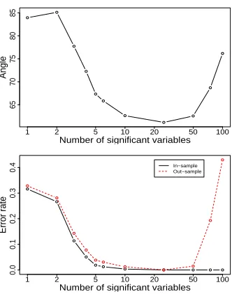
sparse LDA is not directly applicable. We thus applied the sparse rLDA to the simulated data sets. Denote the number of significant variables involved in specifying the discriminant direction to bem. For each of 50 simulated data sets, we applied sparse rLDA for m= 1, 2, 3, 4, 5, 10, 20, 30, 40, 50, 75, 100, and calculated the angles be-tween the estimated and the true discriminant directions. The average angles as a function of m is plotted in the top panel of Figure 3. It is very clear that sparsity helps: Compare average angles around 30 degrees for m = 2– 20 to an average angle about 60 degrees for m = 100. Sparse discriminant vectors are closer to the theoretical direction than the non-sparse ones.
The theoretical discriminant direction has only 2 nonzero components, while in Figure 3 the smallest average an-gle is achieved when m = 10. Although difference of the average angles between m = 2 and m = 10 is not significant, one may wonder why m= 10 is the best in-stead of m= 2. The main reason for this discrepancy is the insufficiency of training sample size, which causes the
1 2 5 10 20 50 100
30
40
50
60
Number of significant variables
Angle
1 2 5 10 20 50 100
0.00
0.10
0.20
0.30
Number of significant variables
Error rate
In−sample Out−sample
Figure 3: A simulated example with two classes. Top panel: The average of angles between the estimated and theoretical directions as a function of the number of vari-ables used. Bottom panel: Average classification error rates using least centroid on the projected data. Based on 50 simulations.
estimation of the covariance matrix Σw inaccurate and
therefore the inclusion of more variables. We did some simulation experiments with increased sample size and observed that the optimal m indeed decrease and come closer tom= 2.
The closeness of estimated direction to the theoretical direction also translates into out-of-sample classification performance. The bottom panel of Figure 3 shows the in-sample and out-of-in-sample classification error rate using nearest centroid method applied to the projected data. When all variables are used in constructing the discrimi-nant vectors, the overfitting of training data is apparent, and is associated with low in-sample error rate and high out-of-sample error rate. The out-of-sample error rate is minimized when the number of significant variables used in constructing the discriminant vectors is ten. It is also interesting to point out that the shape of the out-of-sample error rate curve resembles that of the average angle curve shown on the top panel of Figure 3.
−4 −2 0 2 4
rLDA training
−4 −2 0 2 4
sparse rLDA training
−4 −2 0 2 4
rLDA test
−4 −2 0 2 4
sparse rLDA test
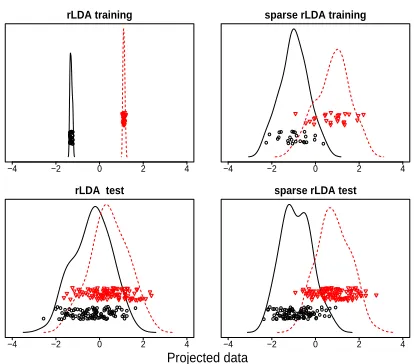
[image:9.612.66.273.55.237.2]Projected data
Figure 4: A simulated example with two classes. Top panels are the results of rLDA and sparse rLDA (m= 5) for the training data; bottom panels are the results for the test data. The in-sample and out-of-sample error rates are 0 and 32% for rLDA and 12% and 13.5% for sparse rLDA, when applying the nearest centroid method to the projected data. The dimension of the data is 100 and there are 25 cases for each class.
On the other hand, if sparsity is imposed in obtaining the discriminant direction, data piling of training set dis-appears and substantial improvement in test set classifi-cation is manifested.
4.2
Three classes
In this example we have three classes. The dimension of the input data is p= 100. For each class, there are 25 cases in the training data set and 200 cases in the test data set. The distribution of each class is
xi∼
N3(µi,Σw,3)
Np−3(0, Ip−3)
, i= 1,2,3,
where
(µ1, µ2, µ3) =
00 −00.9.9 00
1.6 1.1 0
and
Σw,3=
10 01 00..77
0.7 0.7 1
.
There are two discriminant directions of Fisher’s LDA for this three-class problem. We first derive the theoretical directions. As in the previous example, we can ignore the redundant variables in this calculation. The between-class covariance matrix is given by
Σb,3=
1 2
3
X
i=1
(µi−µ¯)(µi−µ¯)T
and the within-class covariance matrix is Σw,3. The
two true projection directions are the eigenvectors of Σ−1
w,3Σb,3.
Since the within-class covariance matrix with all variables is singular, we applied sparse rLDA to the simulated data sets. There are two discriminant directions that form a 2-dimensional dimension reduction subspace. In estimat-ing the sparse discriminant directions, we let the number of included variablesm in the two projections to be the same. For a set of values of m, we calculated the an-gles between the estimated projection subspace and the theoretical discriminant subspace for 50 simulation runs. Here the angle between two q-dimensional spaces is de-fined byθ= arccos(ρ), whereρ is the vector correlation coefficient (Hotelling 1936) defined in the following way. SupposeA andB are two matrices whose columns form the orthonormal bases of the two q-dimensional spaces under consideration. Then the vector correlation coeffi-cient is
ρ=
q
Y
i=1
ρ2i
1/2
,
where ρ2
i are the eigenvalues of the matrix BTAATB.
The top panel of Figure 5 shows the average angles as a function ofm, while the bottom panel shows the error rate of nearest centroid applied to the projected data. Both the average angle and the out-of-sample error rate is minimized aroundm= 30. Use of only a small number of variables in constructing the discriminant directions does help estimate the theoretical directions more accurately and improve the classification performance.
To illustrate the discriminant power using estimated dis-criminant directions, we show in Figure 6 the projection of a training data set and a test data set on the subspace spanned by the two discriminant directions obtained us-ing rLDA and sparse rLDA. Without incorporatus-ing spar-sity in the discriminant vector, the data piling is apparent in training data set and projected data lead to terrible discrimination. As a contrast, if sparsity is imposed in estimating the discriminant directions, the data piling in the training set is avoided and good test set classification is achieved.
5
Real Data Examples
5.1
Wine data
analy-1 2 5 10 20 50 100
65
70
75
80
85
Number of significant variables
Angle
1 2 5 10 20 50 100
0.0
0.1
0.2
0.3
0.4
Number of significant variables
Error rate
[image:10.612.86.252.76.287.2]In−sample Out−sample
Figure 5: A simulated example with three classes. Top panel: The average of angles between the estimated and theoretical directions as a function of the number of vari-ables used. Bottom panel: Average classification error rates using least centroid on the projected data. Based on 50 simulations.
−3 −2 −1 0 1 2 3
−2
0
2
4
rLDA training
Direction 1
Direciton 2
−1.0 −0.5 0.0 0.5 1.0 1.5 2.0
−1
0
1
2
sparse rLDA training
Direction 1
Direciton 2
−3 −2 −1 0 1 2 3
−2
0
2
4
rLDA test
Direction 1
Direciton 2
−1.0 −0.5 0.0 0.5 1.0 1.5 2.0
−1
0
1
2
sparse rLDA test
Direction 1
Direciton 2
Figure 6: A simulated example with three classes. Top panels are the results of rLDA and sparse rLDA (m= 10) for the training data; bottom panels are the results for the test data. The in-sample and out-of-sample error rates are 0 and 44.3% for rLDA and 0 and 0.3% for sparse rLDA, when applying the nearest centroid method to the projected data. The dimension of the data is 100 and for each class, there are 25 cases in the training data and 200 cases in the test data.
sis is to find which type of wine a new sample belonging to based on its 13 attributes. The data consists of 178 instances, each belonging to one of three classes. This is not a HDLSS setting. Fisher’s LDA projects the data to a two-dimensional subspace of R13. We would like to explore if it is possible to classify the wines using only part of the 13 constituents. In estimating the sparse dis-criminant directions, for simplicity, we let both direction vectors to have the same number of nonzero components m, which is set between 1 and 13.
We partitioned the data randomly into a training set with 2/3 of the data and a test set with 1/3 of the data. We did the random partition 50 times to average out the variability in the results due to the partition. For each partition, we used sparse LDA on the training data and obtained two sparse discriminant directions. Then we used the nearest centroid method on the projected data and computed the test set error rates. Figure 7 shows the average of error rates for 50 partitions as a function of the number of variables involved in each estimated sparse direction.
0 2 4 6 8 10 12 14
0.05
0.10
0.15
0.20
0.25
number of variables
[image:10.612.322.526.348.481.2]test error rates
Figure 7: Wine data. The average of error rates as a function of the number of variables. Based on 50 random partitions of the dataset into training and test.
From the plot it is clear that if we specify m = 6 for each discriminate direction, sparse LDA can discriminate the classes fairly well. To check the stability of variable selection, we fixedm= 6, did 50 random partitions, and recorded the selected variables for each partition. Table 1 summarizes the frequency of each variable being selected. It shows that the variable selection is not sensitive to the random partition. Overall, eight variables are important in the discriminant analysis.
[image:10.612.63.270.412.580.2]Table 1: Wine data. Frequency of selected variables.
P P
P P
P P
PP
variable♯
1 2 3 4 5 6 7 8 9 10 11 12 13
projection 1 1 11 0 50 45 0 50 0 0 50 0 43 50
projection 2 50 49 2 48 45 0 1 0 4 49 0 2 50
importance √ √ √ √ √ √ √ √
the data almost as well as using all the variables. It is not surprising that the separation is the best when using all the variables because, in this example, each variable is a constituent that characterizes the wine and would not be redundant. But the sparse LDA does suggest which constituents are the most important in the classification of wines.
−6 −5 −4 −3 −2 −1
3
4
5
6
7
LDA training
direction 1
direciton 2
−4 −2 0 2
12
14
16
18
20
22
sparse LDA training
direction 1
direciton 2
−6 −5 −4 −3 −2 −1
3
4
5
6
7
LDA test
direction 1
direciton 2
−4 −2 0 2
12
14
16
18
20
22
sparse LDA test
direction 1
direciton 2
Figure 8: Wine data. Projection of the data (training and test separately) onto the two discriminant directions.
5.2
Gene expression data
We use two gene expression microarray data sets to il-lustrate the sparse rLDA method. Gene expression mi-croarrays can be used to discriminate between multiple clinical and biological classes. It is a typical example of HDLSS settings because there are usually thousands of genes while the availability of the patients is very limited.
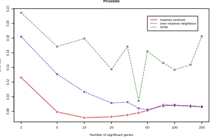
The first data set is the Colon data set (Alon et al., 1999), which contains 42 tumor and 20 normal colon tissue sam-ples. For each sample there are 2000 gene expression level measurements. The second data set is the Prostate data set (Singh et al., 2002), which contains 52 tumor samples and 50 normal samples. For each sample there exist 6033 gene expression level measurements. For both data sets, the goal of the analysis is classification of tumor and nor-mal samples based on the gene expression measurements.
2 5 10 20 50 100 200
0.16
0.18
0.20
0.22
0.24
0.26
Colon
Number of significant genes
Error rate
[image:11.612.326.528.184.308.2]nearest centroid one−nearest neighbour SVM
Figure 9: Colon data. The average test error rate as a function of the number of significant genes for the nearest centroid, 1-nearest neighbor and support vector machine, applied to the reduced data obtained from sparse rLDA. Based on 50 (2:1) training-test partition of the original data set.
For each data set, we first reduce the dimensionality of the data by projecting the data to the discriminant di-rections obtained using sparse rLDA, then the reduced data is used as an input to some standard classification methods. We shall examine the effect of gene selection on classification. Our sparse rLDA algorithm incorpo-rates gene selection to constructing discriminant vector. To expedite computation, we implemented a two-step procedure. First we do a crude gene preselection using the Wilcoxon rank test statistic to obtain 200 significant genes. Then the preselected gene expressions are used as input to sparse rLDA. Note that even after gene prese-lection, we still have HDLSS settings, so regularization of with-in class covariance matrices is needed and the sparse rLDA instead of the sparse LDA algorithm should be applied.
[image:11.612.62.271.280.433.2]2 5 10 20 50 100 200
0.08
0.10
0.12
0.14
0.16
0.18
0.20
0.22
Prostate
Number of significant genes
Error rate
[image:12.612.65.272.64.200.2]nearest centroid one−nearest neighbour SVM
Figure 10: Prostate data. The average test error rate as a function of the number of significant genes for the nearest centroid, 1-nearest neighbor and support vector machine, applied to the reduced data obtained from sparse rLDA. Based on 50 (2:1) training-test partition of the original data set.
the misclassification error rate was computed. To reduce variability, the splitting into training and test sets were repeated 50 times and the error rate is averaged. It is important to note that, for reliable conclusion, all gene preselection, applying sparse rLDA and fitting classifiers were re-done on each of the 50 training sets.
Three classifiers, the nearest centroid, 1-nearest neighbor and support vector machine, have been applied to the re-duced data for classification. Figures 9 and 10 plot the average test error rate as a function of significant genes used in sparse rLDA for the two data sets. The x-axis is plotted using the logarithmic scale to put less focus on large values. As the number of significant genes vary from 2 to 200, the error rates for three methods all de-crease first and then rise. The nearest centroid method has the best overall classification performance. The ben-eficial effect of variable selection in sparse rLDA is clear: The classification using reduced data based on sparse dis-criminant vectors perform better than that based on non-sparse discriminant vectors. For example, if the nearest centroid method is used as the classifier, using the sparse discriminant vectors based on only 10-20 significant genes gives the best test set classification, while using all 200 genes is harmful to classification. Note that the 200 genes used are preselected significant genes, the benefit of using the sparse rLDA could be much bigger if the 200 genes were randomly selected.
6
Conclusions
In this paper, we propose a novel algorithm for con-structing sparse discriminant vectors. The sparse dis-criminant vectors are useful for supervised dimension re-duction for high dimensional data. Naive application of
classical Fisher’s LDA to high dimensional, low sample size settings suffers from the data piling problem. Intro-ducing sparsity in the discriminant vectors is very effec-tive in eliminating data piling and the associated over-fitting problem. Our results on simulated and real data examples suggest that, in the presence of irrelevant or redundant variables, the sparse LDA method can select important variables for discriminant analysis and thereby yield improved classification.
Acknowledgments
Jianhua Z. Huang was partially supported by grants from the National Science Foundation (DMS-0606580) and the National Cancer Institute (CA57030). Lan Zhou was par-tially supported by a training grant from the National Cancer Institute.
Reference
1. Ahn, J. and Marron, J.S., 2007, The maximal data piling direction for discrimination, manuscript.
2. Alon, U., Barkai, N., Notterman, D., Gish, K., Mack, S. and Levine, J., 1999, Broad patterns of gene ex-pression revealed by clustering analysis of tumor and normal colon tissues probed by ologonucleotide ar-rays,Proc. Natl. Acad. Sci, USA,96, 503-511.
3. Campbell, N.A., 1980, Shrunken estimator in dis-criminant and canonical variate analysis, Applied
Statistics,29, 5-14.
4. Cliff, N., 1966, Orthogonal rotation to congruence.
Psychometrika,31, 33-42.
5. Efron B., Hastie T., Johnstone, I., and Tibshirani, R., 2004, Least angle regression, Ann. Statist., 32, 407-499.
6. Fisher, R. A., 1936, The use of multiple measure-ments in taxonomic problems. Ann. Eugen, 7, 179-188.
7. Friedman, J. H., 1989, Regularized discriminant analysis, Journal of the American Statistical
Asso-ciation,84, 165-175.
8. Gower, J. C. and Dijksterhuis, G. B., 2004, Pro-crustes Problems, Oxford University Press, New York.
9. Hotelling, H., 1933, Analysis of a complex of statis-tical variables into principal components. J. Educ.
Psych.,24, 417-441, 498–520.
11. Fukunaga, K., 1990, Introduction to Statistical Pat-tern Classification. Academic Press, San Diego, Cal-ifornia, USA, 1990.
12. Mardia, K.V., Kent, J.T. and Bibby J.M., 1979, Multivariate analysis,Academic Press.
13. Marron, J. S., Todd, M. and Ahn, J., 2007, Distance weighted discrimination, Journal of American
Sta-tistical Association,102, 1267–1271.
14. Pearson, K., 1901, On lines and planes of closest fit to systems of points in space, Philosophical Maga-zine,2, 559-572.
15. Peck, R. and Van Ness, J., 1982, The use of shrink-age estimators in linear discriminant analysis,IEEE Transactions on Pattern Analysis and Machine
In-telligence,4, 531-537.
16. Rayens, W.S., 1990, A Role for covariance stabiliza-tion in the construcstabiliza-tion of the classical mixture sur-face,Journal of Chemometrics,4, 159-169.
17. Singh, D., Febbo, P. G., Ross, K., Jackson, D. G., Manola, J., Ladd, C., Tamayo, P., Renshaw, A. A., D’Amico, A.V., Richie, J. P., Lander, E. S., Loda, M., Kantoff, P., W., Golub, T. R., and Sellers, W. R., 2002, Gene expression correlates of clinical prostate cancer behavior,Cancer Cell,1, 203-209.
18. Tibshirani, R., 1996, Regression shrinkage and se-lection via the lasso,Journal of the Royal Statistical
Society, Series B,58, 267-288.
19. Ye, J., 2005, Characterization of a family of algo-rithms for generalized discriminant analysis on un-dersampled problems,Journal of Machine Learning
Research,6, 483-502.
20. Ye, J., Janardan, R., Li, Q. and Park H., 2006, Feature reduction via generalized uncorrelated lin-ear discriminant analysis, emphIEEE Transactions on Knowledge and Data Engineering,18, 1312-1322.
21. Zou, H., Hastie, T. and Tibshirani, R., 2006, Sparse principal component analysis, Journal of