Quantitative Analysis of
Local Adaptive Thresholding Techniques
M. Chandrakala
Assistant Professor, Department of ECE, MGIT, Hyderabad, Telangana, India
ABSTRACT: Thresholding is a simple but effective technique for image segmentation. In this paper, a general locally adaptive thresholding method using neighborhood processing is presented. The method makes use of local image statistics of mean and variance within a variable neighborhood and two thresholds obtained from the global intensity distribution. This paper describes local adaptive thresholding techniques that remove background by using local mean and standard deviation. Normally the local mean computational time depends on the window size. The locally adaptive thresholding algorithms were tested with images including noise and non uniform illumination. The results were compared with a number of locally adaptive techniques qualitatively in the literature. Locally adaptive thresholding works with great success even in cases of with poor quality, shadows, non uniform illumination, low contrast, large signal-dependent noise, smear and strain. In order to demonstrate the effectiveness, locally adaptive thresholding had been implemented in printed text and real world images.
KEYWORDS: Image thresholding; Image segmentation; window size; ME; FPNR; standard deviation; Image variance
I. INTRODUCTION
Thresholding is an important technique in image segmentation and machine vision applications. A survey of thresholding methods and their applications exist in literature [1].Thresholding techniques can be divided into global and local thresholding depending on the number of thresholds required to be detected. Local thresholding methods can deal with non-uniform illumination but they are complicated and slow. Among the global thresholding techniques, the study concluded that [2] the Otsu method [3] was one of the better threshold selection methods for general real world images with uniform illumination. The renowned Otsu's [3] method suggests minimizing the weighted sum of variances of the objects and background pixels to establish an optimum threshold. But it is clear that a fixed value of threshold value cannot give satisfactory results.
Local threshold method performs better in case of badly illuminated images and document image analysis as threshold computation is dependent on region characteristics. NiBlack[4] method the mean and standard deviation to compute threshold over a small window). Bernsen [5] uses mean and standard deviation along with contrast information to compute a threshold for a certain region adaptive contribution of standard deviation in determining local threshold. Parker [6] uses slightly different approach to solve bad illumination problem and compute local threshold value by classifying object and background pixels and then using region growing to produce a binarized image. Locally adaptive thrsholding techniques like Bernsen [5], Niblack [4], Sauvola and Pietikainen [7] and Feng’s method [8] estimate a different threshold for each pixel according to the grayscale information of the neighbouring pixels. In local thresholding, the thresholding value is varied based on local content of image.
Different binarization methods have been evaluated in [3, 4, 5, 7, 8] for different types of images. In this paper, we present quantitative evaluation of locally adaptive binarization methods for gray scale images with low contrast, variable background intensity and noise. In that evaluation, Niblack’s method [4] was found to be the better of them all. Different improvements have since been made to the original Niblack method to improve the results. These include Sauvola’s algorithm [7], Bernsen [5], Niblack [4] and Feng’s method [8].
Feng’s method [8]. Section 3 discusses experimental results for the selected adaptive threshold methods. Finally, Conclusion is drawn in section 4.
II. REVIEW OF SELECTED THRESHOLDING TECHNIQUES
In this section, we briefly review the Otsu method for selecting optimal image threshold. Since the thresholding is done once for the whole image,one may lose certain local characteristics. Locally adaptive threshold based methods Sauvola’s algorithm [7], Bernsen [5], Niblack [4] and Feng’s method [8], are characterized by calculation of threshold at every pixel.
A. The Otsu method
One of the threshold based techniques that was widely used is Otsu method [3]. This method works on gray scale image and selects an optimal threshold value automatically from a gray level histogram. First, it is simple and has the ability to process the gray level mages directly. Second, it is able to work with a global threshold values due to its low sensitivity to dark areas [9]. Finally, the method covers a wide scope of unsupervised decision procedure where it does not require training images in order to get prior knowledge about the histogram shape [10]. This process requires high computational time especially for images that were classified into a large number of classes. Furthermore, the usage of Otsu technique alone in the application was not enough to produce accurate segmentation result especially for images under uneven lighting condition [11].
B. Niblack’s Technique
Niblack[4] is a local thresholding algorithm that adapts the threshold according to the local mean and the local standard deviation over a specific window size around each pixel location. The local threshold at any pixel (i, j) is calculated as:
T (i, j) = m (i, j) +k σ (i, j) (1)
Where m (i, j) and σ (i, j) are the local sample mean and standard deviation, respectively. The size of the local region (window) is dependent upon the application. The value of the weight 'k' is used to control and adjust the effect of standard deviation due to objects features. Niblack algorithm suggests the value of 'k' to be -0.2. The document images binarized using the Niblack algorithm provides the most satisfactory results. Niblack fails to adapt large variation in illumination, especially in the document images. The local region analysis using Niblack does not provide any kind of information about the global attributes of the image that may be helpful in the v process of badly illuminated images. Another problem it faces is the optimum selection of the weight ‘k’.
C. Sauvola Technique
Local-variance-based robust method is proposed by Sauvola [7]. This approach calculates local threshold value using local mean and local standard deviation for each pixel separately. With Sauvola’s method, the background noise problem that appears in Niblack’s approach is solved but in many cases where there are less intensity variations; characters become extremely thinned and broken. In some cases, the characters disappear totally giving a white output image. This method gives improvement over the method proposed by Niblack, especially when the background contains light texture, big variations, stained and badly and unevenly illuminated documents. It adapts the contribution of the standard deviation.
( , ) = ( , )∗ 1 + ( , )−1 (2)
The typical suggested value for k = 0.5 and R = 128. Here m is mean and is ′ ′ standard deviation of the entire
window. The value of k and window size gives large effect on quality of image. The drawback of method is, reactive to the selection of window size and free parameter values and computationally slow. However, in images where the gray values of text and non-text pixels are close to each other, the results degrade significantly.
The modified Local adaptive method proposed by Bernsen [5] which estimates the local threshold with mean value of minimum and maximum intensities of pixels within a window. The threshold value is set using midrange intensity value of pixel within a local window, which is the mean of the minimum I (i, j) and maximum I (i, j) of gray values.
C(i, j) = I (i, j)−I (i, j) (3)
Where C(i, j) denotes the contrast of an image pixel (i, j). The pixel will be sort into text or background by comparing minimum and maximum intensities. If the local contrast C(i, j) is smaller than the threshold then the pixel is appoint as background and vice-versa. The method, not perform well on degraded document images with a complex background. Local threshold value depends on the mean value of the minimum and maximum intensities of pixels in a window. It does not perform well with a complex background. However, if the contrast C (i,j) is below a certain threshold , then that neighborhood is said to consist of only one class, foreground or background. There is no bias to control the threshold value.
E. Feng’s technique
Feng et al. [8] proposed a local thresholding technique. This method considers two local windows which is one contained within other (i.e. primary and secondary window). It locally calculates gray value standard deviation from whole image using both windows. To find the threshold value ‘T’, The values of local mean ‘m’, the minimum gray-level ‘M’, and standard deviation ‘S’ are calculated in the primary local window while the dynamic range standard deviation Rs is calculated in the larger window termed as ‘secondary local window’. Binarization threshold is then
computed as:
= (1− )∗ + ∗ ∗( − ) + ∗ (4)
Where = and = Based on the experimental experiences of authors, is set to 2 while the values of other parameters , proposed to be in the ranges 0.1-0.2, 0.15-0.25 and 0.01-0.05 respectively. Feng’s method generally works very well but the main drawback remains its susceptibility to the empirically determined parameter values as discussed earlier. A slight change in parameter values could drastically affect the binarization results. One set of parameter values could give excellent results for one image but the same set would not work for another image with different intensity and illumination variations. Secondly, the introduction of a larger secondary window (around the primary window) also makes this method computationally inefficient as compared to the rest.
III. RESULTS AND ANALYSIS
We have considered five images with non-uniform illumination condition having different sizes, airpalne1 image (256×256),field image(256×256),bird image(256×256), airplane2 image (256×256) print document image(493x1153), images are shown in Fig. 1(a) to 5(a).The corresponding ground truth images from Berkeley data set(real world images ) and DIBCO -2009 (Printed document ) is shown in Fig. 1(h) to 5(h). All the experiments are performed in MATLAB 14.0.
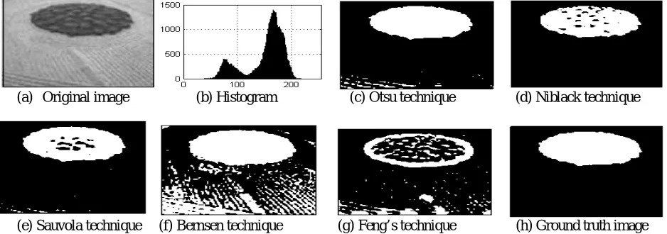
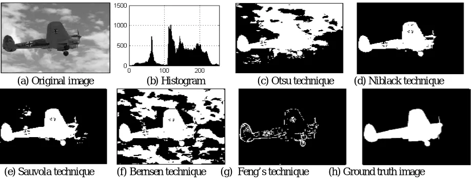
(e) Sauvola technique (f) Bernsen technique (g) Feng’s technique (h) Ground truth image Fig. 1: (a) Original image of airplane1, (b) Histogram of image, (c) Otsu technique (d) Niblack technique (e) Sauvola technique, (f) Bernsen technique, (g) Feng’s technique and (h) Ground truth image
Fig. 1(a) Shows airplane 1 image and fig. 1(h) shows the corresponding ground-truth image. The airplane 1 image consists of object and backgrounds with different gray level distribution range. As a result, the gray level histogram of the image is unimodal distribution as shown in fig. 1(b). Object gray values are identical to the part of background gray values there by misclassified background pixels appear in the foreground in Otsu method as shown in fig.1(c). In local adaptive thresholding algorithms, depending on application the size of window and coefficient ‘k’ changes from image to image. We selected window size as 200x200 and ‘k’= -0.0005.However the segmentation accuracy is better compared to Otsu as shown in fig. 1(d). In Sauvola thresholding method for airplane 1 image, window size as 40x40 and ‘k’= 0.03. However the segmentation misclassified pixels in Sauvola method very less compared to above selected segmentation methods is shown in fig. 1(e). In Bernsen thresholding method we selected window size as 323x323 and ‘k’= -0.05, segmented result of airplane1 image is over segmented compared to all remaining methods as shown in fig 1(f). Feng thresholding segmented result of airplane1 image is under segmented compared to all remaining methods as shown in fig 1(g).
(a) Original image (b) Histogram (c) Otsu technique (d) Niblack technique
(e) Sauvola technique (f) Bernsen technique (g) Feng’s technique (h) Ground truth image Fig. 2: (a) Original image of field, (b) Histogram of image, (c) Otsu technique, (d) Niblack technique
(e) Sauvola technique, (f) Bernsen technique, (g) Feng’s technique and (h) Ground truth image
(a)Original image (b) Histogram (c) Otsu technique (d) Niblack technique
(e) Sauvola technique (f) Bernsen technique (g) Feng’s technique (h) Ground truth image Fig. 3: (a) Original image of bird, (b) Histogram of image, (c) Otsu technique (d) Niblack technique
(e) Sauvola technique, (f) Bernsen technique, (g) Feng’s technique and (h) Ground truth image
Bird image and the corresponding ground-truth images are displayed in Fig. 3(a), fig. 3(h) respectively. The Bird image contains object and background with different gray levels. As a result, the gray level histogram of the image is unimodal distribution as shown in fig. 3(b).Top right corner gray levels of background identical to some part of object gray levels in bird image as shown in fig. 3(a). Inaccurate segmentation at tail part of the bird using otsu as shown in fig.3(c). Niblack uses window size as 200x200 and ‘k’= -0.0005, segmentation result as shown in fig. 3(d). Sauvola method uses window size as 50x50 and ‘k’= 0.3, segmentation result as shown in fig. 3(e). Bernsen thresholding method, background left corner and right corner pixels segmented in to foreground as shown in fig 3(f). Feng mehod is under segmented as shown in fig.3 (g).
(a) Original image (b) Histogram (c) Otsu technique (d) Niblack technique
(e) Sauvola technique (f) Bernsen technique (g) Feng’s technique (h) Ground truth image
Fig. 4: (a) Original image of airplane2, (b) Histogram of image, (c) Otsu technique (d) Niblack technique (e) Sauvola technique, (f) Bernsen technique, (g) Feng’s technique and (h) Ground truth image
Bernsen is over segmented as compared to other thresholding methods as shown in fig. 4(f). Feng is under segmented as compared to other selected thresholding methods as shown in fig. 4(g).
(a) Original image (b) Histogram (c) Otsu technique (d) Niblack technique
(e) Sauvola technique (f) Bernsen technique (g) Feng’s technique (h) Ground truth image
Fig. 5: (a) Original image of printed text, (b) Histogram of image, (c) Otsu technique (d) Niblack technique (e) Sauvola technique, (f) Bernsen technique, (g) Feng’s technique and (h) Ground truth image
Printed text image and the corresponding ground-truth images are displayed in Fig. 5(a), fig. 5(h) respectively. The printed text image contains object and background with different gray level distribution range. As a result, the gray level histogram of the image is unimodal distribution as shown in fig. 5(b). Otsu thresholding only few misclassified background pixels appears in the foreground as shown in fig. 5(c). For text images, the window sizeis required to change depending on the character size. Otherwise only the character boundary is detected for large character size. The value of k is used to adjust how much of the total print object boundary is taken as a part of the given object. We selected window size as 200x200 and ‘k’= -0.0005, Niblack thresholding produces a large amount of black noise in the empty windows as shown in fig.5 (d). Sauvola thresholding misclassified more numbers of pixels than Niblack as shown in fig.5 (e). Bernsen method contains noise pixels under segmented result as shown in fig.5 (f) compared to other thresholding methods. Feng method is under segmented as shown in Fig. 5(g).
In the experiments we tested the performance of Otsu, Sauvola’s algorithm, Bernsen, Niblack and Feng’s method using quantitative measures. For each experiment we have evaluated misclassification error, false positive rate and false negative rate. The quality of image segmentation was quantitatively evaluated via three measures: misclassification error (ME) [12], false positive rate (FPR) and false negative rate (FNR) [13]. For two-class segmentation, Misclassification error can be simply formulated as
= 1−| ∩ | + | ∩ |
+ | | (5)
B0indicates the background of the original image and F0 indicates the foreground of the original image. BT and FT
denote the background and foreground of the test image. The ME measures the percentage of the background which is misclassified as the foreground and conversely, the foreground which is being misclassified as the background. A lower value of misclassification error means better quality. FPR is the rate of the number of background pixels misclassified into foreground pixels to the total number of background pixels in the ground truth image. Similarly, FNR is the rate of the number of foreground pixels misclassified into background pixels to the total number of foreground pixels in the ground truth image. For two-class segmentation, FPR and FNR can be respectively formulated as
=| ∩ |
=| ∩ |
| | (7)
The values of FPR and FNR also vary between 0 and 1. FPR and FNR indicate over-segmentation and under segmentation, respectively. High values of FPR and FNR correspond to serious over-segmentation and under-segmentation, respectively. In our practical calculations of FPR and FNR, we assumed that the size of object is smaller than that of background in an image.
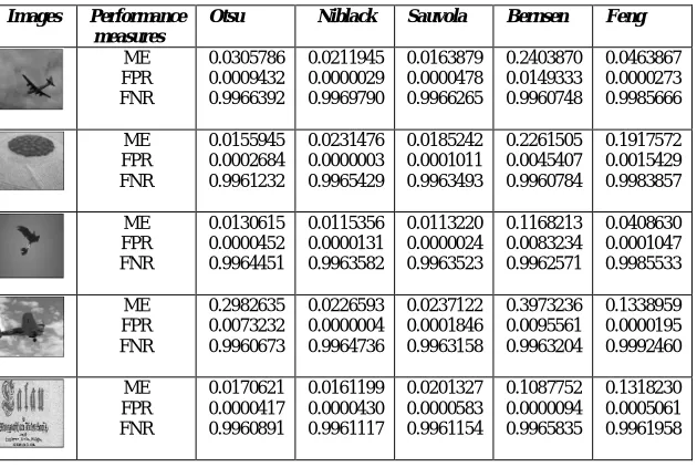
Experimental results are listed in Table 1. In addition, the table compares ME for five different images with simple, Otsu, Niblack, Sauvola, Bernsen and Feng’s thresholding techniques. A smaller ME value indicates better value of thresholding for segmentation. Moreover by analyzing the results reported in Table 1, airplane1 image ME is less in Sauvola algorithm than other methods. Field image ME is less in Otsu method than other methods. Bird image ME is less in Sauvola technique than other methods. Airplane2 image ME is less in Niblack algorithm than other methods. Printed document image ME is less in Niblack algorithm than other methods. After analysis we conclude that ME is reduced for field image and printed document image in Niblack technique as compared to remaining techniques.ME is reduced for airplane1image and bird image in Sauvola technique as compared to remaining techniques. From experimental analysis we conclude that for non uniform and noisy images Sauvola technique and Niblack technique can easily separate object from back ground
Table 1
Quantitative comparison on ME, FPR and FNR for the images
Images Performance
measures
Otsu Niblack Sauvola Bernsen Feng
ME FPR FNR 0.0305786 0.0009432 0.9966392 0.0211945 0.0000029 0.9969790 0.0163879 0.0000478 0.9966265 0.2403870 0.0149333 0.9960748 0.0463867 0.0000273 0.9985666 ME FPR FNR 0.0155945 0.0002684 0.9961232 0.0231476 0.0000003 0.9965429 0.0185242 0.0001011 0.9963493 0.2261505 0.0045407 0.9960784 0.1917572 0.0015429 0.9983857 ME FPR FNR 0.0130615 0.0000452 0.9964451 0.0115356 0.0000131 0.9963582 0.0113220 0.0000024 0.9963523 0.1168213 0.0083234 0.9962571 0.0408630 0.0001047 0.9985533 ME FPR FNR 0.2982635 0.0073232 0.9960673 0.0226593 0.0000004 0.9964736 0.0237122 0.0001846 0.9963158 0.3973236 0.0095561 0.9963204 0.1338959 0.0000195 0.9992460 ME FPR FNR 0.0170621 0.0000417 0.9960891 0.0161199 0.0000430 0.9961117 0.0201327 0.0000583 0.9961154 0.1087752 0.0000094 0.9965835 0.1318230 0.0005061 0.9961958
Quantitative comparison on false positive rate for the images as shown in table 1, In addition, the table compares FPR for five different images with simple, Otsu, Niblack, Sauvola, Bernsen and Feng thresholding techniques. A larger FPR value indicates over segmentation. Moreover by analyzing the results reported in Table 1, airplane1 image FPR is more in Bernsen algorithm than other methods. In Field image FPR is more in Bernsen method than other methods. Bird image FPR is more in Bernsen technique than other methods. Airplane2 image FPR is more in Bernsen technique than other methods. Printed document image FPR is more in Sauvola algorithm than other methods. After analysis we conclude that FPR is more in Bernsen thresholding technique for all images except printed document image as compared to remaining techniques.
After analysis we conclude that FNR is more in Feng’s algorithm in all images except printed document image as compared to remaining techniques.
.V.CONCLUSION
In this paper,we present the quantitative analysis of various methods for comparison. Performance varies at different window size. Niblack’s and Bernsen’s methods require large window size. For certain images, these two techniques are not suitable at smaller window size. Adaptive thresholding methods, computational time depend on window size. For document images, the window size is required to change depending on the character size. Niblack method gives better result than other methods. Feng’s algorithm is under segmented than other methods. Bernsen thresholding is over segmented than other methods.
REFERENCES
1. M. Sezgin, B. Sankur, “Survey over image thresholding techniques and quantitative performance evaluation”, J.Electronic Imaging, Vol. 13 (1),
pp. 146–165, 2004.
2. P.K. Sahoo, S.Soltani, A.K.C.Wong, Y.C.Chen. “A survey of thresholding techniques”, Compute Vision”, Graphics, and Image Processing, Vol.41, Issue 2., pp. 233–260, 1988.
3. N. Otsu, "A threshold selection methods from grey-level histograms”, IEEE transactions on systems, man and cybernetics, Vol SMC-9, Issue 1, pp.162-66, 1979.
4. W.Niblack, "An Introduction to Digital Image Processing", Engle wood. Cliffs, N.J. Prenlice Hall, pp. 115-1 16, 1956.
5. J.Bernsen, “Dynamic thresholding of grey-level images”, Proc. 8th International Conference on Pattern Recognition (ICPR8), pp.1251-1255,
Paris, 1986.
6. J. K. Parker, "Gray level thresholding in badly illuminated images" .IEEE Transactions on Pattern Analysis and Machine Intelligence,
Volume 13, pp. 813-819, August 1991.
7. J. Sauvola, T. Seppanen, S. Haapakoski and M. Pietikainen, “Adaptive document binarization”. Proc. 4th Int. Conf. on Document Analysis and Recognition, pp. 147–152, Ulm Germany, 1997.
8. Meng-Ling Feng and Yap-Peng Tan, “Contrast adaptive binarization of low quality document images”, IEICE, Vol.16, pp.501-506.
9. U. G. Barron and F. Butler, "A comparison of seven thresholding techniques with the k- means clustering algorithm for measurement of
bread-crumb features by digital image analysis," Journal of Food Engineering, Vol.74, pp. 268-278, 2006.
10. J. W. Funck, Y. Zhong, D. A. Butler, C. C. Brunner, and J. B. Forrer, "Image segmentation algorithms applied to wood defect detection", Computers and Electronics in Agriculture, Vol. 41, pp. 157-179, 2003.
11. Q. Huang, W. Gao, W. Cai, "Thresholding technique with adaptive window selection for uneven lighting image", Pattern Recognition Letters, Vol. 26, pp. 801-808.
12. W.A. Yasnoff, J.K. Mui, J.W. Bacus, “Error measures for scene segmentation”, Pattern Recognition, Vol.3, pp. 217–231.
13. Hu, Q., Zujun Hou, and W. L. Nowinski, "Supervised range-constrained thresholding.", IEEE Trans Image Process, vol. 15, issue 1, pp. 228-40, 2006.
BIOGRAPHY