Discrete time bifurcation behavior of a prey predator system with generalized predator

(1)

R E S E A R C H

Open Access

Discrete-time bifurcation behavior of a

prey-predator system with generalized

predator

Harkaran Singh

1*

_{, Joydip Dhar}

2

_{and Harbax Singh Bhatti}

3

*_{Correspondence:}

harkaran78@yahoo.in

1_{Department of Applied Sciences,}

Khalsa College of Engineering and Technology, Amritsar, Punjab 143001, India

Full list of author information is available at the end of the article

Abstract

In the present study, keeping in view of Leslie-Gower prey-predator model, the stability and bifurcation analysis of discrete-time prey-predator system with generalized predator (i.e., predator partially dependent on prey) is examined. Global stability of the system at the fixed points has been discussed. The specific conditions for existence of flip bifurcation and Neimark-Sacker bifurcation in the interior ofR2

+ have been derived by using center manifold theorem and bifurcation theory.

Numerical simulation results show consistency with theoretical analysis. In the case of a flip bifurcation, numerical simulations display orbits of period 2, 4, 8 and chaotic sets; whereas in the case of a Neimark-Sacker bifurcation, a smooth invariant circle bifurcates from the fixed point and stable period 16, 26 windows appear within the chaotic area. The complexity of the dynamical behavior is confirmed by a

computation of the Lyapunov exponents.

Keywords: prey-predator system; center manifold theorem; ﬂip bifurcation; Neimark-Sacker bifurcation; Lyapunov exponent; chaos

1 Introduction

It is a well recognized fact that the prey-predator interaction is a subject of great interest in the bio-mathematical literature and the dynamic relationship between predator and prey living in the same environment will continue to be one of the important themes in mathematical ecology (Berryman [], Lotka [], May [], Volterra []). Many researchers studied the dynamical behavior of the prey-predator system in ecology and contributed to the growth of the population models [–].

Liu [] investigated the existence of periodic solutions for a discrete semi-ratio-dependent prey-predator model. Huo and Li [] obtained conditions for the global sta-bility of solutions for a delayed discrete prey-predator system with the help of Lyapunov functions. Chen [] proposed a discrete prey-predator system and obtained conditions for the global stability of an equilibrium for non-autonomous and periodic cases. Liaoet al.[] investigated a one-predator two-prey discrete model and derived the conditions for the local asymptotic stability of equilibrium of the system. Fan and Li [] established suﬃcient conditions in a delayed discrete prey-predator model with Holling type III func-tional response for permanence. However, there are few articles discussing the dynamical

(2)

behavior of discrete-time prey-predator models for exploring the possibility of bifurca-tions and chaos phenomena [–].

In the present study, motivated by the Leslie-Gower prey-predator model [, ], we propose a discrete-time prey-predator system with predator partially dependent on prey [] and investigate the stability and bifurcation analysis of the system by using center manifold theorem and bifurcation theory. This paper is organized as follows: in Section , we obtained fixed points of the discrete-time system and discussed the stability criterion of the system at the fixed points. In Section , the specific conditions of the existence of a flip bifurcation and a Neimark-Sacker bifurcation are derived. Finally, in Section , numerical simulations are carried out to support our analytical findings, especially for period doubling bifurcation and chaotic behavior.

The prey-predator system is of the form

_dx

dt =ax( – x k) –

bxy x+l, dy

dt = [ – my nx+q–d]y,

()

wherex(t) andy(t) represent the densities of prey and predator populations, respectively. Again, the parameteradenote the intrinsic growth rate of prey;bis harvesting rate of prey by predator;ddenotes the death rate of predator;kdenotes carrying capacity of the prey in a particular habitat;ldenotes the half saturation constant;mis the maximum value which per capita reduction rate of predator can attend;nis a measure of the food quality that the prey provides for conversion into predator births;qis the extent to which alternatives are provided for the growth of predator.

Applying the forward Euler scheme to the system of equations (), we obtain the discrete-time prey-predator system:

x→x+δ[ax( –x_k) –bxy_x₊_l],

y→y+δ[ –_nxmy₊_q–d]y, ()

whereδis the step size. The numerical solution to the initial value problem obtained from Euler’s method with step sizeδ, and the total number of steps N satisﬁes  <δ≤ L

N,

whereLis the length of the interval.

2 Stability of ﬁxed points

The ﬁxed points of the system () areO(k, ),A(,(–_md)q) andB(x∗,y∗), wherex∗,y∗satisfy

a( –x_k∗) –_xby∗₊∗_l= ,

 –_nxmy∗₊∗_q–d= .

()

The Jacobian matrix of () at the ﬁxed point (x,y) is written as

J=

⎡

⎣ +δ(a–axk – bly

(x+l)) –

bδx

(x+l)

δmny

(nx+q)  +δ( – my nx+q–d)

⎤ ⎦.

The characteristic equation of the Jacobian matrix is given by

(3)

where

p(x,y) = –trJ= – –δ

 +a–d–ax

k – bly

(x+l) – my nx+q

,

q(x,y) =detJ

=  +δ

a–ax

k – bly

(x+l)  +δ

 – my

nx+q–d

+ δ

_bmnxy

(x+l)(nx+q).

Now, we state a lemma similar to [, ].

Lemma . Let F(λ) =λ+Bλ+C.Suppose that F() > ;λandλare roots of F(λ) = . Then we have:

(i) |λ|< and|λ|< if and only ifF(–) > andC< ;

(ii) |λ|< and|λ|> (or|λ|> and|λ|< )if and only ifF(–) < ;

(iii) |λ|> and|λ|> if and only ifF(–) > andC> ;

(iv) λ= –and|λ| = if and only ifF(–) = andB= , ;

(v) λandλare complex and|λ|=|λ|= if and only ifB– C< andC= .

Letλandλbe the roots of (), which are known as eigen values of the ﬁxed point (x,y).

The ﬁxed point (x,y) is a sink or locally asymptotically stable if|λ|<  and|λ|< . The

ﬁxed point (x,y) is a source or locally unstable if|λ|>  and|λ|> . The ﬁxed point (x,y)

is non-hyperbolic if either|λ|=  or|λ|= . The ﬁxed point (x,y) is a saddle if|λ|> 

and|λ|<  (or|λ|<  and|λ|> ).

Proposition . The ﬁxed point O(k, )is source ifδ> _a,saddle if <δ< _a,and non-hyperbolic ifδ=_a.

One can see that whenδ=_a, one of the eigen values of the ﬁxed pointO(k, ) is – and magnitude of other is not equal to . Thus the ﬂip bifurcation occurs when the parameter changes in a small neighborhood ofδ=_a.

Proposition . There exist diﬀerent topological types of A(,(–_md)q)for possible parame-ters.

(i) A(,(–_md)q)is sink ifbq( –d) >almand <δ<min{_–_d,_bq_(–_dlm_)–_alm}. (ii) A(,(–_md)q)is source ifbq( –d) >almandδ>max{_–_d,_bq_(–_dlm_)–_alm}.

(iii) A(,(–_md)q)is non-hyperbolic ifbq( –d) >almand eitherδ=_–_dorδ=_bq_(–_dlm_)–_alm. (iv) A(,(–_md)q)is saddle for all values of the parameters,except for that values which lies

in(i)to(iii).

The term (iii) of Proposition . implies that the parameters lie in the set

FA=

(a,b,d,k,l,m,n,q,δ),δ=   –d,δ=

lm

bq( –d) –almand

bq( –d) >alm,a,b,d,k,l,m,n,q,δ> 

(4)

If the term (iii) of Proposition . holds, then one of the eigen values of the ﬁxed point

A(,(–_md)q) is – and the magnitude of the other is not equal to . The pointA(,(–_md)q) undergoes a ﬂip bifurcation when the parameter changes in small neighborhood ofFA.

The characteristic equation of the Jacobian matrixJof the system () at the ﬁxed point

B(x∗,y∗) is written as

λ+px∗,y∗λ+qx∗,y∗= , ()

where

px∗,y∗= – –Gδ,

qx∗,y∗=  +Gδ+Hδ

and

G=  +a–d–ax

∗

k –

bly∗

(x∗+l)– my∗ nx∗+q,

H= a–ax

∗

k –

bly∗

(x∗+l)  –

my∗ nx∗+q–d

+ bmnx

∗_y∗

(x∗+l)(nx∗+q).

Now

F(λ) =λ– ( +Gδ)λ+ +Gδ+Hδ.

Therefore

F() =Hδ, F(–) =  + Gδ+Hδ.

Using Lemma ., we get the following proposition.

Proposition . There exist diﬀerent topological types of B(x∗,y∗)for all possible param-eters.

(i) B(x∗,y∗)is a sink if either condition(i.)or(i.)holds: (i.) G– H≥and <δ<–G–

√

G_–_H

H ,

(i.) G_{– }_H_{< }_and_{ <}_δ_{< –}G H.

(ii) B(x∗,y∗)is source if either condition(ii.)or(ii.)holds: (ii.) G– H≥andδ>–G+

√

G_–_H

H ,

(ii.) G_{– }_H_{< }_and_δ_{> –}G H.

(iii) B(x∗,y∗)is non-hyperbolic if either condition(iii.)or(iii.)holds: (iii.) G– H≥andδ=–G±

√

G_–_H

H ,

(iii.) G_{– }_H_{< }_and_δ_{= –}G H.

(iv) B(x∗,y∗)is saddle for all values of the parameters,except for that values which lies in (i)to(iii).

If the term (iii.) of Proposition . holds, then one of the eigen values of the ﬁxed point

(5)

Proposi-tion . may be written as follows:

If the term (iii.) of Proposition . holds, then the eigen values of the ﬁxed point

B(x∗,y∗) are a pair of complex conjugate numbers with modulus . The term (iii.) of Proposition . may be written as follows:

HB=

In this section, we study the ﬂip bifurcation and the Neimark-Sacker bifurcation at the ﬁxed pointB(x∗,y∗).

Consider the perturbation of ()

(6)

(7)

+[b( +a) +ab]δ

Applying the center manifold theorem to () at the origin in the limited neighborhood ofδ∗= . The center manifoldWc_{(, ) can be approximately represented as}

Wc(, ) =(x˜,y˜) :˜y=aδ∗+ax˜+ax˜δ∗+aδ∗+O

|˜x|+δ∗,

whereO((|˜x|+|δ∗|)) is a function with at least third orders in variables (x˜,δ∗). By simple calculations for the center manifold, we have

a= ,

Now, consider the map restricted to the center manifoldWc_{(, ) as below:}

(8)

According to the ﬂip bifurcation, the discriminatory quantitiesγandγare given by

γ=

∂f ∂x˜∂δ∗ +

 

∂f ∂δ∗

∂f ∂x˜

(,)

,

γ=

 

∂_f ∂x˜+

 

∂_f ∂x˜



(,)

.

After simple calculations, we obtainγ=handγ=h+h.

Analyzing the above and the ﬂip bifurcation conditions discussed in [], we write the following theorem.

Theorem . Ifγ= ,and the parameterδ∗alters in the limiting region of the point(, ), then the system()passes through a ﬂip bifurcation at the point B(x∗,y∗).Also,the

period-points that bifurcate from the ﬁxed point B(x∗,y∗)are stable(resp.,unstable)ifγ> 

(resp.,γ< ).

3.2 Neimark-Sacker bifurcation

Consider the system () with arbitrary parameter (a,b,d,k,l,m,n,q,δ)∈HB, which is

de-scribed as follows:

x→x+δ[ax( –x_k) –bxy_x₊_l], y→y+δ[ –_nxmy₊_q–d]y.

()

B(x∗,y∗) is a ﬁxed point of the system (), wherex∗,y∗are given by () and

δ= – G H.

Consider the perturbation of ()

x→x+ (δ+δ)[ax( –x_k) –bxy_x₊_l], y→y+ (δ+δ)[ –_nxmy₊_q–d]y,

()

where|δ|  is limited perturbation parameter.

The characteristic equation of map () atB(x∗,y∗) is given by

λ+p(δ)λ+q(δ) = ,

where

p(δ) = – –G(δ+δ),

q(δ) =  +G(δ+δ) +H(δ+δ).

Since the parameters (a,b,d,k,l,m,n,q,δ)∈HB, the eigen values ofB(x∗,y∗) are a pair

of complex conjugate numbersλandλwith modulus  by Proposition ., where

λ,λ=–p(δ)∓i

q(δ) –p₍_δ₎

(9)

(10)

where

According to the Neimark-Sacker bifurcation, the discriminatory quantitysis given by

s= –Re ( – λ)λ

Analyzing the above and the Neimark-Sacker bifurcation conditions discussed in [], we write the theorem as follows.

Theorem . If the condition()holds,s= and the parameterδalters in the limited region of the point(, ),then the system()passes through a Neimark-Sacker bifurcation at the point B(x∗,y∗).Moreover,if s<  (resp.,s> ),then an attracting(resp.,repelling)

invariant closed curve bifurcates from the ﬁxed point B(x∗,y∗)forδ>  (resp.,δ< ).

4 Numerical simulations

(11)

Figure 1 Bifurcation diagram and largest Lyapunov exponents of the system (2) fora= 0.2,b= 0.12,

d= 0.14,k= 4,l= 3,m= 0.1,n= 0.2,q= 0.5, andδcovering [2.3, 3.2].

(., .). We discuss the following two cases by keeping the parametersb= .,k= ,

l= ,m= .,n= .,q= . as ﬁxed and varying the parametersa,donly.

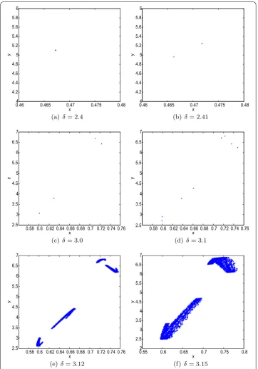
Case: In this case, we takea= .,d= . and obtainγ= –. andγ= .. From

Figure (a), it is observed that the ﬁxed point (., .) of the system () is stable for

δ< ., loses its stability, and a ﬂip bifurcation appears atδ= .. It shows that The-orem . is true.

The phase portraits show that there are orbits of period , ,  atδ= ., ., ., respec-tively, and chaotic sets atδ= ., . (see Figure ). Moreover, the largest Lyapunov expo-nents corresponding toδ= . and . are positive, conﬁrming the existence of chaotic sets (see Figure (b)).

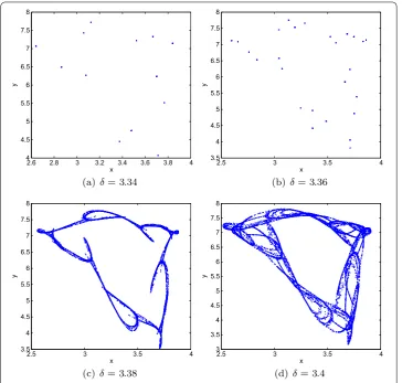
Case: In this case, we takea= .,d= . and obtains= –.. From Figure (a), it is observed that the ﬁxed point (., .) of the system () is stable for δ< ., loses its stability, and a Neimark-Sacker bifurcation emerges atδ= .. It indicates that Theorem . is satisﬁed.

The phase portraits in Figures  and  show that a smooth invariant circle bifurcates from the ﬁxed point (., .) and its radius increases with the increase of δ. There are windows of period ,  atδ= ., ., respectively, and chaotic attractors atδ= . and .. Moreover, the largest Lyapunov exponents corresponding toδ= . and . are positive, conﬁrming that we have chaotic sets (see Figure (b)).

5 Conclusions

In this paper, we investigated the stability and bifurcation analysis of discrete-time prey-predator system with prey-predator partially dependent on prey in the closed first quad-rantR₊. The map undergoes a flip bifurcation and a Neimark-Sacker bifurcation at the fixed point under specific conditions whenδvaries in a small neighborhood ofFBorFB

andHB. Numerical simulations of the model display orbits of period , ,  and chaotic

(12)

(13)

Figure 3 Bifurcation diagram and largest Lyapunov exponents of the system (2) fora= 0.8,b= 0.12,

d= 0.44,k= 4,l= 3,m= 0.1,n= 0.2,q= 0.5, andδcovering [2.9, 3.5].

(14)

Figure 5 Phase portraits for several values ofδfrom 3.34 to 3.4 related to Figure 3(a).

Competing interests

The authors declare that they have no competing interests.

Authors’ contributions

All authors read and approved the manuscript.

Author details

1_{Department of Applied Sciences, Khalsa College of Engineering and Technology, Amritsar, Punjab 143001, India.} 2_{Department of Applied Sciences, ABV - Indian Institute of Information Technology and Management, Gwalior,}

MP 474015, India.3_{Department of Applied Sciences, B.B.S.B. Engineering College, Fatehgarh Sahib, Punjab 24105, India.}

Acknowledgements

The authors would like to thank the referee and reviewer for their constructive suggestions on improving the presentation of the paper.

Received: 2 April 2015 Accepted: 17 June 2015 References

1. Berryman, AA: The origins and evolution of predator-prey theory. Ecology73(5), 1530-1535 (1992) 2. Lotka, AJ: Elements of Physical Biology (1925)

3. May, RM: Stability and Complexity in Model Ecosystems, vol. 6. Princeton University Press, Princeton (2001) 4. Volterra, V: Fluctuations in the abundance of a species considered mathematically. Nature118, 558-560 (1926) 5. Agrawal, T, Saleem, M: Complex dynamics in a ratio-dependent two-predator one-prey model. Comput. Appl. Math.

34, 265-274 (2015)

6. Alebraheem, J, Hasan, YA: Dynamics of a two predator-one prey system. Comput. Appl. Math.33, 767-780 (2014) 7. Dhar, J: A prey-predator model with diﬀusion and a supplementary resource for the prey in a two-patch

environment. Math. Model. Anal.9(1), 9-24 (2004)

(15)

9. Dubey, B: A prey-predator model with a reserved area. Nonlinear Anal., Model. Control12(4), 479-494 (2007) 10. Freedman, H: Deterministic Mathematical Models in Population Ecology. HIFR Consulting Ltd, Edmonton (1980) 11. Jeschke, JM, Kopp, M, Tollrian, R: Predator functional responses: discriminating between handling and digesting prey.

Ecol. Monogr.72(1), 95-112 (2002)

12. Kooij, RE, Zegeling, A: A predator-prey model with Ivlev’s functional response. J. Math. Anal. Appl.198(2), 473-489 (1996)

13. Ma, W, Takeuchi, Y: Stability analysis on a predator-prey system with distributed delays. J. Comput. Appl. Math.88(1), 79-94 (1998)

14. Sen, M, Banerjee, M, Morozov, A: Bifurcation analysis of a ratio-dependent prey-predator model with the Allee eﬀect. Ecol. Complex.11, 12-27 (2012)

15. Sinha, S, Misra, O, Dhar, J: Modelling a predator-prey system with infected prey in polluted environment. Appl. Math. Model.34(7), 1861-1872 (2010)

16. Murray, JD: Mathematical Biology I: An Introduction. Interdisciplinary Applied Mathematics, vol. 17. Springer, New York (2002)

17. Robinson, C: Dynamical Systems: Stability, Symbolic Dynamics, and Chaos. CRC Press, Boca Raton (1998)

18. Agarwal, RP: Diﬀerence Equations and Inequalities: Theory, Methods, and Applications. CRC Press, Boca Raton (2000) 19. Agarwal, RP, Wong, PJ: Advanced Topics in Diﬀerence Equations. Springer, Berlin (1997)

20. Celik, C, Duman, O: Allee eﬀect in a discrete-time predator-prey system. Chaos Solitons Fractals40(4), 1956-1962 (2009)

21. Dhar, J, Singh, H, Bhatti, HS: Discrete-time dynamics of a system with crowding eﬀect and predator partially dependent on prey. Appl. Math. Comput.252, 324-335 (2015)

22. Gopalsamy, K: Stability and Oscillations in Delay Diﬀerential Equations of Population Dynamics. Springer, Berlin (1992) 23. Guckenheimer, J, Holmes, P: Nonlinear Oscillations, Dynamical Systems, and Bifurcations of Vector Fields. Applied

Mathematical Sciences, vol. 42. Springer, New York (1983)

24. Liu, X, Xiao, D: Complex dynamic behaviors of a discrete-time predator-prey system. Chaos Solitons Fractals32(1), 80-94 (2007)

25. Liu, X: A note on the existence of periodic solutions in discrete predator-prey models. Appl. Math. Model.34(9), 2477-2483 (2010)

26. Huo, HF, Li, WT: Existence and global stability of periodic solutions of a discrete predator-prey system with delays. Appl. Math. Comput.153(2), 337-351 (2004)

27. Chen, F: Permanence and global attractivity of a discrete multispecies Lotka-Volterra competition predator-prey systems. Appl. Math. Comput.182(1), 3-12 (2006)

28. Liao, X, Zhou, S, Ouyang, Z: On a stoichiometric two predators on one prey discrete model. Appl. Math. Lett.20(3), 272-278 (2007)

29. Fan, YH, Li, WT: Permanence for a delayed discrete ratio-dependent predator-prey system with Holling type functional response. J. Math. Anal. Appl.299(2), 357-374 (2004)

30. Chen, Y, Changming, S: Stability and Hopf bifurcation analysis in a prey-predator system with stage-structure for prey and time delay. Chaos Solitons Fractals38(4), 1104-1114 (2008)

31. Gakkhar, S, Singh, A: Complex dynamics in a prey predator system with multiple delays. Commun. Nonlinear Sci. Numer. Simul.17(2), 914-929 (2012)

32. He, Z, Lai, X: Bifurcation and chaotic behavior of a discrete-time predator-prey system. Nonlinear Anal., Real World Appl.12(1), 403-417 (2011)

33. Hu, Z, Teng, Z, Zhang, L: Stability and bifurcation analysis of a discrete predator-prey model with nonmonotonic functional response. Nonlinear Anal., Real World Appl.12(4), 2356-2377 (2011)

34. Jing, Z, Yang, J: Bifurcation and chaos in discrete-time predator-prey system. Chaos Solitons Fractals27(1), 259-277 (2006)

35. Zhang, CH, Yan, XP, Cui, GH: Hopf bifurcations in a predator-prey system with a discrete delay and a distributed delay. Nonlinear Anal., Real World Appl.11(5), 4141-4153 (2010)

36. Leslie, P: Some further notes on the use of matrices in population mathematics. Biometrika35, 213-245 (1948) 37. Leslie, P: A stochastic model for studying the properties of certain biological systems by numerical methods.

Biometrika45, 16-31 (1958)