R E S E A R C H
Open Access
Global dynamics of cubic second order
difference equation in the first quadrant
Jasmin Bekteševi´c
1, Mustafa RS Kulenovi´c
2*and Esmir Pilav
3*Correspondence:
2Department of Mathematics,
University of Rhode Island, Kingston, Rhode Island 02881-0816, USA Full list of author information is available at the end of the article
Abstract
We investigate the global behavior of a cubic second order difference equation
xn+1=Axn3+Bxn2xn–1+Cxnxn2–1+Dx3n–1+Ex2n+Fxnxn–1+Gx2n–1+Hxn+Ixn–1+J, n= 0, 1,. . ., with nonnegative parameters and initial conditions. We establish the relations for the local stability of equilibriums and the existence of period-two solutions. We then use this result to give global behavior results for special ranges of the parameters and determine the basins of attraction of all equilibrium points. We give a class of examples of second order difference equations with quadratic terms for which a discrete version of the 16th Hilbert problem does not hold. We also give the class of second order difference equations with quadratic terms for which the Julia set can be found explicitly and represent a planar quadratic curve.
MSC: Primary 39A10; 39A11; 65L12; 65L20; secondary 37E99; 37D10
Keywords: basin of attraction; competitive map; global stable manifold; monotonicity; period-two solution
1 Introduction and preliminaries
In this paper we study the global dynamics of the following polynomial difference equa-tion:
xn+=Axn+Bxnxn–+Cxnxn–+Dxn–+Exn+Fxnxn–+Gxn–+Hxn+Ixn–+J, ()
where the parametersA,B,C,D,E,F,G,H,I,Jare nonnegative numbers with condition A+B+C+D> and initial conditionsx–andxare arbitrary nonnegative numbers.
The conditionA+B+C+D> is necessary in order to avoid the quadratic case, which was completely studied in []. Polynomial difference equations and corresponding maps have been studied in both the real and the complex domain and many results have been obtained; see [–]. One of the major problems in the dynamics of polynomial maps is determining the basin of attraction of the point at∞and in particular the boundary of that basin known as the Julia set. In [] we precisely determined the Julia set for a second order quadratic polynomial equation, that is, () whereA+B+C+D= , and we obtained the global dynamics in the interior of the Julia set, which includes all the point for which solutions are not asymptotic to the point at∞. It turned out that the Julia set for (), where A+B+C+D= , is the union of the stable manifolds of some saddle equilibrium points or nonhyperbolic equilibrium points or period-two points. The asymptotic formulas for
these manifolds were obtained in []. The advantage of our results is that these manifolds are continuous decreasing functions of which the parametrization is simple and so their asymptotic formulas can easily be derived by using the method of undetermined coeffi-cients.
In this paper we restrict our attention to nonnegative initial conditions and nonnegative parameters, which will make our results more special but also more precise and applica-ble. Our results are based on a number of theorems which hold for monotone difference equations, which will be described in the next section. Our principal tool is the theory of monotone maps, and in particular cooperative maps, which guarantee the existence and uniqueness of the stable and unstable manifolds for the fixed points and periodic points. Our results can be extended to () to hold in the whole plane, whenB=C=E=F=G= .
Remark The following result is a consequence of our results in []: IfA=B=C=D= E=H=J= ,F=G> andI< , then (), which reduces to the quadratic second order difference equation
xn+=F
xnxn–+xn–
+Ixn–, n= , , . . . ,
has infinitely many minimal period-two solutions, which are given by
H=(x,y) :F(x+y) +I= ,x> ,y> .
The curveHseparates the first quadrant into two regions: the region below the curveHis the basin of attraction ofE(, ) and the region above the curve is the basin of attraction
of point at infinity. Thus, the curveHis the Julia set for () in this case. This result shows that the discrete version of the th Hilbert problem does not hold, which is the problem if there exists a quadratic system of difference equations in the plane with an infinite number of periodic solutions. It is well known that in the case of quadratic systems of differential equations the number of periodic solutions is finite; see [, ]. In this paper we give the explicit formula for the Julia set for a whole class of difference equations with cubic terms. The Julia set consists of an infinite number of period-two solutions and thus provides the whole class of examples of the second order difference equations with the cubic terms with an infinite number of a period-two solutions; see Theorem .
The rest of this section presents some results as regards monotone difference equations in the plane. The second section presents the local stability analysis of the equilibrium solutions. The third section describes the local stability analysis of the period-two points in all cases. The fourth section gives the global dynamics, which includes the basins of attraction of all equilibrium points and the period-two points. SomeMathematicaoutputs are given in the Appendix.
Consider the difference equation
xn+=f(xn,xn–), n= , , . . . , ()
wheref is a continuous and increasing function in both variables.
Theorem Let f: [a,b]×[a,b]→[a,b]be a continuous function satisfying the following properties:
(i) f(x,y)is nondecreasing in each of its arguments,i.e.x→f(x,y)is nondecreasing for everyyandy→f(x,y)is nondecreasing for everyx;
(ii) ()has a unique equilibriumx∈[a,b]. Then every solution of()converges to x.
The following result was obtained in [].
Theorem Let I⊆Rbe an interval(finite or infinite)and let f ∈C[I×I,I]be a function which increases in both variables.Then for every solution of ()the subsequences{xn}∞n=
and{xn+}∞n=–of even and odd terms of the solution do exactly one of the following:
(i) Eventually they are both monotonically increasing. (ii) Eventually they are both monotonically decreasing.
(iii) One of them is monotonically increasing and the other is monotonically decreasing.
As a consequence of Theorem every bounded solution of () approaches either an equilibrium solution or period-two solution or the singular point on the boundary and every unbounded solution is asymptotic to the point at infinity in a monotonic way; see []. Thus the major problem in the dynamics of () is the problem of determining the basins of attraction of three different types of attractors: the equilibrium solutions, period-two solution(s), and the point(s) at infinity. The following period-two results can be proved by using the techniques of the proof of Theorem in [].
Theorem Consider()where I⊆Ris an interval(finite or infinite)and f ∈C[I×I,I] is an increasing function in its arguments and assume that there is no minimal period-two solution.Assume that E(x,y)and E(x,y)are two consecutive equilibrium points in
North-East ordering that satisfy
(x,y)ne(x,y)
and that E is a local attractor and E is a saddle point or a nonhyperbolic point with
second characteristic root in the interval(–, ),with the neighborhoods where f is strictly increasing.Then the basin of attractionB(E)of E is the region below the global stable
manifoldWs(E
).More precisely
B(E) =
(x,y) :∃yu:y<yu, (x,yu)∈Ws(E)
.
The basin of attractionB(E) =Ws(E)is exactly the global stable manifold of E.The
global stable manifold extends to the boundary of the domain of().If there exists a period-two solution,then the end points of the global stable manifold are exactly the period-two solution.
Also, we will use the following theorem from [].
solution.Assume that E(x,y),E(x,y),and E(x,y)are three consecutive equilibrium
points in North-East ordering that satisfy
(x,y)ne(x,y)ne(x,y)
and that Eand Eare saddle points with the neighborhoods where f is strictly increasing,
and Eis a local attractor.Then the basin of attractionB(E)of Eis the region between
The following result gives the necessary and sufficient condition for the local stability of () whenf is nondecreasing in all its arguments; see [].
Theorem Let
two polynomials of degreesnandm, respectively. Their resultant (see [–])Res(f,g)
is the determinant of the (m+n)×(m+n) Sylvester matrix given by
(i) The discriminant offis given by
Dis(f) = (–)n(n–)/
an
Resf,f
and
Dis(f·g) =Dis(f)Dis(g)Res(f,g),
wheref is the derivative off.
(ii) Dis(f) = ⇔fhas a double root inC:Equivalently,fhas n distinct roots inCif
and only if the discriminant is= .
For two bivariate polynomialsf,g∈R[x,y], Theorem in [, ] holds.
Theorem Let f(x,y),g(x,y)∈R[x,y]where
f(x,y) = n
i=
fi(x)yi and g(x,y) = m
i=
gi(x)yi,
and let r(x) =Resy(f,g)∈R[x]be the resultant of f and g with respect to the variable y. Then:
(a) f andghave a nontrivial common factor if and only ifris identically zero. (b) Iff andgare co-prime(do not have a common factor),the following conditions are
equivalent:
• α∈Cis a root ofr.
• fn(α) =gm(α) = or there isβ∈Cwithf(α,β) = =g(α,β) = . (c) For all(α,β)∈C×C:iff(α,β) = =g(α,β) = ,thenr(α) = .
We list some results when solution{xn}of () tends to the point at infinity in a monotonic way.
Theorem If H+I> ,then every solution{xn}of()satisfieslimn→∞xn=∞.
Proof If{xn}is a solution of (), then{xn}satisfies the inequality
xn+≥Hxn+Ixn–, n= , , . . . ,
which in view of the result on difference inequalities, see Theorem .. in [], implies thatxn≥yn,n≥, where{yn}is a solution of the initial value problem
yn+=Hyn+Iyn–, y–=x– and y=x n= , , . . . .
Consequently,
xn≥yn= √
H+ I
(Ix–+λx)λn+ (λx–+Ix)λn
, n= , , . . . ,
where
λ,=
H±√H+ I
and λ<λ and λ> ,
Theorem If J≥,then every solution{xn}of()satisfieslimn→∞xn=∞.
Proof LetJ≥ and setA+B+C+D+E+F+G+H+I=α> . If{xn}is a solution of (), thenxn>Jforn≥, and by using the fact that the function
f(x,y) =Ax+Bxy+Cxy+Dy+Ex+Fxy+Gy+Hx+Iy+J
is increasing in both variables we obtain the following result:
f(J,J) = (A+B+C+D)J+ (E+F+G)J+ (H+I)J+J
≥(A+B+C+D)J+ (E+F+G)J+ (H+I)J+J
= (A+B+C+D+E+F+G+H+I+ )J= ( +α)J
and
x=f(x,x) >f(J,J)≥( +α)J,
x=f(x,x) >f(J,J)≥( +α)J,
x=f(x,x) >f
( +α)J, ( +α)J≥( +α)J, x=f(x,x) >f
( +α)J, ( +α)J≥( +α)J, ..
.
Continuing in this way we obtain
xn+> ( +α)nJ and xn+> ( +α)nJ for alln≥,
which impliesxn+→ ∞andxn+→ ∞.
Theorem If A+B+C+D+E+F+G+H+I> or J> and A+B+C+D+E+F+ G+H+I≥,then the box[,∞)is a part of the basin of attraction of the point at infinity
of().
Proof Set
A+B+C+D+E+F+G+H+I=k≥
and
f(x,y) =Ax+Bxy+Cxy+Dy+Ex+Fxy+Gy+Hx+Iy+J. ()
Clearly, the functionf(x,y) is increasing in both variables. Ifx,y∈[,∞), then
f(x,x) = (A+B+C+D)x+ (E+F+G)x+ (H+I)x+J
≥(A+B+C+D)x+ (E+F+G)x+ (H+I)x+J
Since the initial conditionsx–,x∈[,∞),
x=f(x,x–)≥f(, ) =k+J,
x=f(x,x)≥f(, ) =k+J,
x=f(x,x)≥f(k+J,k+J)≥k(k+J) +J=k+kJ+J,
x=f(x,x)≥f(k+J,k+J) >k+kJ+J,
x=f(x,x)≥f
k+kJ+J,k+kJ+J≥kk+kJ+J+J=k+kJ+kJ+J, x=f(x,x)≥f
k+kJ+J,k+kJ+J≥kk+kJ+J+J=k+kJ+kJ+J. An immediate application of mathematical induction yields
xn–≥kn+
kn–+kn–+· · ·+ J,
xn>kn+
kn–+kn–+· · ·+ J
for alln≥. Ifk> , thenkn→ ∞and ifk= thenkn–+kn–+· · ·+ → ∞. In both cases
we getxn–→ ∞andxn→ ∞.
Theorem If (H +I – ) < J(E +F +G), then every solution {xn} of () satisfies
limn→∞xn=∞.
Proof If{xn}is a solution of (), then{xn}satisfies the inequality
xn+≥Exn+Fxnxn–+Gxn–+Hxn+Ixn–+J, n= , , . . .
which in view of the result on difference inequalities, see Theorem .. in [], implies thatxn≥yn,n≥ where{yn}is a solution of the initial value problem
yn+=Eyn+Fynyn–+Gyn–+Hyn+Iyn–+J,
y–=x– and y=x, n= , , . . . .
()
Equation () has no equilibrium solutions if and only if
(H+I– )< J(E+F+G).
In view of the results for () in [], see Lemma , there is no prime period-two solution when (H+I– )≤J(E+F+G) orE≥GorH+I> . So if there is no equilibrium point
and there is no prime period-two solution of (), then every solution{yn}of () satisfies
limn→∞yn=∞, which implieslimn→∞xn=∞.
solutions will be following on their way to ∞. In general, it is clear from the proof of Theorem that the escape region of () is a subset of the escape region of (). In the subsequent sections we will consider global dynamics of () in the complement of the parametric region described by Theorems , , , and .
2 Local stability analysis of equilibrium solutions
The equilibrium solutions of () are the nonnegative solutions of the equation
(A+B+C+D)x+ (E+F+G)x+ (H+I– )x+J= . ()
Define the functiong(x) such that
g(x) = (A+B+C+D)x+ (E+F+G)x+ (H+I– )x+J, ()
so the nonnegative solutions ofg(x) = are the nonnegative equilibrium solutions of ().
2.1 The caseJ> 0
Sinceg(–∞) = –∞andg() =J> , we always have one negative root, which means that there are at most two nonnegonnegative equilibrium solutions. The first derivative ofg(x) is
g(x) = (A+B+C+D)x+ (E+F+G)x+ (H+I– ). ()
Denote bythe discriminant of quadratic equationg(x) = , that is,
= (E+F+G)– (A+B+C+D)(H+I– ). ()
We have:
(i) If < , theng(x) > for allxand the functiong(x) is monotonically increasing, which implies that there is no nonnegative root ofg(x) = .
(ii) If= , then
H+I– = (E+F+G)
(A+B+C+D)≥.
Thus,g(x) > for allx≥, which implies that () has no positive solutions. (iii) If> , then for the rootsx,=–(E+F+G)±
√
(A+B+C+D) (x<x) ofg(x) = we get the
fol-lowing:
x+x= –
E+F+G A+B+C+D≤,
which means that at leastxis negative, and
xx=
H+I–
A+B+C+D. ()
• IfH+I> , then () has no positive solutions.
example when the values of parameters are
A+B+C+D= , E+F+G=
The calculation ofg(x) gives
g(x) = x so we always have the zero equilibrium. Denote bydiscriminant of quadratic equation
(A+B+C+D)x+ (E+F+G)x+ (H+I– ) = , ()
that is
The following statements are immediate:
(i) If< , then the zero equilibrium is the only equilibrium.
(ii) If= , then a solution of the quadratic equation () is given by
x= – E+F+G (A+B+C+D).
IfE+F+G> there is no positive solution.E+F+G= impliesH+I= , and again the zero equilibrium is the only equilibrium.
(iii) If> , then for equilibriumsx,=–(E+F+G)± √
(A+B+C+D) (x<x) we havex< and
xx=
H+I– A+B+C+D.
Now, we see that the following statements hold: (a) IfH+I> , then () has no positive solutions.
(b) IfH+I= , thenx= , and there is no positive equilibrium solutions.
(c) IfH+I< , then the only positive equilibrium solution isx.
The equilibrium solutionsx¯of () satisfy the cubic equation (). This immediately shows that there exists a zero equilibriumx¯= if and only ifJ= . The linearized equation at the zero equilibrium is
zn+=Hzn+Izn–. ()
In view of Theorem and the local stability theorem from [] we obtain the following result on the local stability of the zero equilibrium.
Proposition The zero equilibrium of()is one of the following: (a) locally asymptotically stable ifH+I< ,
(b) nonhyperbolic and locally stable ifH+I= , (c) unstable ifH+I> ,
(d) a saddle point ifH>|I– |, (e) a repeller if –I<H<I– .
A necessary condition for the existence of the positive equilibrium(s) isH+I< . The linearized equation at the positive equilibrium solutionsxis
zn+=pzn+qzn–, ()
where
p= (A+ B+C)x+ (E+F)x+H,
q= (B+ C+ D)x+ (F+ G)x+I,
and
Now,
p+q=g(x) + ,
where g(x) is given by (). Letx andx (x<x) be the roots ofg(x) = . By applying
Theorem and the local stability theorem from [] we obtain the following result on the local stability of the positive equilibrium(s).
Proposition The positive equilibrium solution of()is one of the following: (a) locally asymptotically stable ifp+q< ,
(b) nonhyperbolic and locally stable ifp+q= , (c) unstable ifp+q> ,
(d) a saddle point ifp>|q– |, (e) a repeller if –q<p<q– .
The next theorems will describe the local stability for the positive equilibrium(s) in more detail.
Theorem Let J∈(,∞)and H+I< ,then:
(a) Ifg(x) < ,then there are two positive equilibrium solutionsx∈(,x)and
x∈(x, +∞)of().Furthermore,xis locally asymptotically stable andxis
unstable.
(b) Ifg(x) = ,then there is one positive equilibrium solutionx=x,which is
nonhyperbolic and locally stable.
Proof
(a) Whenx∈(,x), theng(x) < , and forx∈(,x) we get
p+q=g(x) + < ,
so by applying Theorem we see thatxis locally asymptotically stable. Whenx∈(x, +∞)
theng(x) > , and forx∈(x, +∞) we get
p+q=g(x) + > ,
so by applying Theorem we see thatxis unstable. By using the Proposition we obtain
the following result:
• xis a saddle point ifq–p< ,
• xis a repeller ifq–p> .
It remains to determineq–pfor equilibriumx:
q–p=(D–A) + (C–B)x+ (G–E)x+I–H.
(b) In this case we have
p+q=g(x) + =g(x) + = ,
Theorem If J= and H+I< andis given by(),then the only positive equilibrium
x+=
–(E+F+G) +√
(A+B+C+D)
of()is unstable.
Proof In this case () has three equilibrium solutionsx–∈(–∞,x),x= , andx+∈(x,∞),
wherexandx(x<x) are the roots ofg(x) = . Now we have
p+q= (A+B+C+D)x++ (E+F+G)x++ (H+I)
=g(x+) + > ,
so by applying Theorem we see thatx+is unstable. By using Proposition we obtain the
following result:
• x+is saddle point ifq–p< ;
• x+is repeller ifq–p> .
It remains to determineq–pfor equilibriumx+:
q–p=(D–A) + (C–B)x++ (G–E)x++I–H. Example It has been shown in [] that the difference equation
xn+=xn+xn–
has one positive equilibriumx+= √
, which is a saddle point. The difference equation
xn+=Axn+Bxnxn–+Cxnxn–+Dxn–+
xn+
xn–
such thatD> A+ B+Chas one positive equilibriumx+=(A+B+C+D). As
q–p=(D–A) + (C–B) (A+B+C+D) +
=
D– A– B–C (A+B+C+D)+ > ,
the positive equilibrium is a repeller.
3 Local stability of period-two solutions
Period-two solutions . . . ,,,,, . . . satisfy the system:
=A+B+C+D+E+F+G+H+I+J, ()
=A+B+C+D+E+F+G+H+I+J. ()
It is clear that if there is a period-two solution it has to beI≤. Also, forH+I> orJ≥ or (H+I– )< J(E+F+G) we have seen thatx
(), () is symmetric, which means that if (,) is a solution of the system (), (), then also (,) is a solution of the system (), (); then we assume without a loss of generality that ≤<. By subtracting () and (), and using the fact that–> , we get
(D–A)(+)+ (A–B+C–D)+ (G–E)(+) +I–H– = . ()
By summing () and () we get
(A+D)(+)+(B+C– A– D)(+)+(E+G)(+)
+ (F–E–G)+(H+I– )(+) + J= . ()
If we set+=x> and=y≥, then () and () yields another system
(D–A)x+ (G–E)x+ (A–B+C–D)y+I–H= , ()
(A+D)x+ (E+G)x+ (B+C– A– D)xy+ (H+I– )x
+ (F–E–G)y+ J= . ()
One can see that the special cases when the period-two solutions do not exist are
H+I>
or
D≤A and A+C≤B+D(orC+D≤A+B) and G≤E.
This immediately leads to the following result.
Theorem Let D≤A,A+C≤B+D(or C+D≤A+B),G≤E,J∈(, ),and H+I< . If≤or> and g(x)∈(,J),then every solution{xn}of()satisfieslimn→∞xn=∞. Here g(x)andare defined by()and(),respectively,and xis the greater root of equation
g(x) = .
Proof SinceH+I< ,D≤A,A+C≤B+D(orC+D≤A+B), andG≤E, we see that () implies that the period-two solutions do not exist. If≤ or> andg(x)∈(,J), then
there is no positive solution ofg(x) = , so there are no positive equilibriums of (). As a consequence of Theorem every bounded solution of () approaches either an equilibrium solution or a period-two solution and every unbounded solution is asymptotic to the point at infinity in a monotonic way. Hence, every solution{xn}of () satisfieslimn→∞xn=∞.
Remark IfD≤A,A+C≤B+D(⇒C≤B),G≤E, then a period-two solution does not exist, so if there exists an unstable positive equilibrium of () we obtain
q–p– =(D–A) + (C–B)x++ (G–E)x++I–H– < ,
Set
un=xn– and vn=xn, n= , , . . .
and write () in the equivalent form:
un+=vn,
The period-two solution is locally asymptotically stable if the eigenvalues of the Jacobian matrixJT, evaluated at (,), lie inside the unit disk. By definition
where
c= ∂f
∂u(,) = A
+ B+C+ E+F+H,
d=∂f
∂v(,) =B
+ C+ D+F+ G+I.
()
Set
S=trJT(,) =
∂g
∂u(,) + ∂h ∂v(,) =a+bc+d≥
and
D=detJT(,) = ∂g
∂u(,) ∂h
∂v(,) – ∂g ∂v(,)
∂h ∂u(,) =a(cb+d) –b(ca) =ad≥.
By applying the linearized stability theorem, the period-two solution (,) is locally asymptotically stable if|S|< +DandD< , that is,
S< +D ⇔ a+bc+d< +ad ⇔ bc< (a– )(d– ) ()
and
D< ⇔ ad< , ()
which implies the following lemma.
Lemma The eigenvalues of the Jacobian matrix of JT at a period-two solution are
non-negative numbers.
In order to solve system of equations () and (), we consider two different cases. (i) IfA+C=B+D, then () becomes the quadratic equation
(D–A)x+ (G–E)x+I–H– = . ()
If D≤AandG≤E, then the period-two solutions do not exist, so at least one of the following inequalities is true:
D>A or G>E.
Also,H+I< impliesI–H– < –H≤. The solutions of the quadratic equation () are given by
x,=
E–G±(E–G)– (D–A)(I–H– )
(a) IfD>A, then (D–A)(I–H– ) < and
x=E–G+
(E–G)– (D–A)(I–H– )
(D–A)
is the only positive solution of (). (b) IfD<A, then () can be written as
(A–D)
positive
x+ (E–G)x+H –I+
positive
= .
It is clear thatE<G. As
xx=
G–E
A–D> and x+x=
H–I+ A–D > ,
when (E–G)> (A–D)(H–I+) we have two positive solutions given by (). If (E–G)=
(A–D)(H–I+ ), then we have one positive solution
x= G–E (A–D).
(c) IfD=A, thenB=C, and () becomes the linear equation
(G–E)x+I–H– = .
IfG=E, thenI=H+ ⇒I≥. CaseH= andI= impliesJ= , so () and () become the same equation,
A++B(+) +E++F= ,
which is impossible for positive,. For positive parameterHwe haveH+I> H+ > , so there is no minimal period-two solution. IfG=E, then
x=
positive
H–I+ G–E ,
in which case we getG>E.
In all the above cases, when (E+G–F) + (A+ D–B–C)x= ,yis given by
y=(A+D)x
+ (E+G)x+ (H+I– )x+ J
(E+G–F) + (A+ D–B–C)x . ()
(ii) IfA+C=B+D, then () gives
y=(D–A)x
+ (G–E)x+I–H–
B+D–A–C ,
and, finally, from () we get the following cubic equation:
where
K=A(C–A) +D(D–B),
K=CE–D(E+F– G) –BG+A(–E+F+G),
K= –D+ (E–G)(E–F+G) –CH+ DH+A( +H– I) +B(– +I) –DI,
K= (F–E–G)(I–H– ) +J(A–B+C–D).
Remark Equation () shows that () can have at most three period-two solutions. Lemma gives an upper bound of the number of period-two solutions of equation () in some special cases. Equation () can be solved but its solutions are very complicated and would depend on parameters. In the remaining part of the paper we will work un-der the assumptions that () has between zero and three period-two solutions and we will present the global dynamics in all possible cases. In particular, Theorem describes a global dynamics in the case when () has one or three period-two solutions, while Theo-rem gives a global dynamics in the case when () has zero or two period-two solutions. The existence of at least one period-two solution is guaranteed by Theorem .
4 Global behavior
In this section we present the global dynamics of () in different parametric regions.
4.1 The case that there exists a minimal period-two solution on the coordinate axes (
= 0 and
> 0)
In this section we consider the special case when= and> . Equation () implies
A+E+H+J= .
Since> , we getA=E=H=J= . Now, from () we obtain
D+G+I– = . ()
IfI= , then we must haveD=G= and∈R+. IfI< , thenis a positive solution of (), that is,
=–G+
G+ D( –I)
D .
Also, ifD= andI< , then
= –I G .
.. The case:A=D=E=G=H=J= ,I=
IfA=D=E=G=H=J= andI= , then (,) = (,t) wheret∈R+is a period-two solution of the difference equation
All other minimal period-two solutions (,) are solutions of the system
=B+C+F+ ,
=B+C+F+ .
One can show that this system has no other positive solutions except (,) = (,t) where
a=Bt+Ft+ , b= , c=Ct+Ft, d= .
Sincebc= (a– )(d– ) orS= +D, the period-two solution is nonhyperbolic. The global behavior of this equation is described in Section and, in this case, every solution goes to infinity.
.. The case:A=E=H=J= and I<
IfA=E=H=J= andI< , then (,) = (,–G+ √
G+D(–I)
D ) is the period-two solution of the difference equation
xn+=Bxnxn–+Cxnxn–+Dxn–+Fxnxn–+Gxn–+Ixn–. ()
All other minimal period-two solutions (,) are solutions of the system
=B+C+D+F+G+I, =B+C+D+F+G+I.
SinceH+I< , there are locally stable zero equilibrium and positive unstable equilibrium.
It is useful to note that ifB=DandF=G, then (,) = (,–F+ √
F+B(–I)
B ) is also a solution of the equation
B++C+F(+) +I– = . In this case every point on the curve
Bx+y+Cxy+F(x+y) +I– = ()
is a period-two solution of () except the equilibrium point (x+,x+).
One can see that for (,) = (,–G+ √
G+D(–I)
D )
a=B+F+I, b= , c=C+F, d= D+ G+I.
Now, we have
(a– )(d– ) =B+F+I– D+ G+I– =B+F+I– D+G +I–
=
+ D+G
and
and for the positive equilibriumx+we obtain
q–p– =D+ (C–B)x++ Gx++I– equilibriumx+is a saddle point.
• In the case whenB+F+I= , then(a– )(d– ) = =bcorS= +D, which the curve()is a period-two solution of (), except the equilibrium point, Since q–p– = , the positive equilibriumx+is a nonhyperbolic point. Also, the points
(,) ={(,–F+ the positive equilibriumx+is a repeller.
One can prove that ifB=D,F=GorF=G,B=Dthe mapT has no other minimal
period-two solutions except (,) = (,–G+ √
G+D(–I)
D ). This leads to the following result.
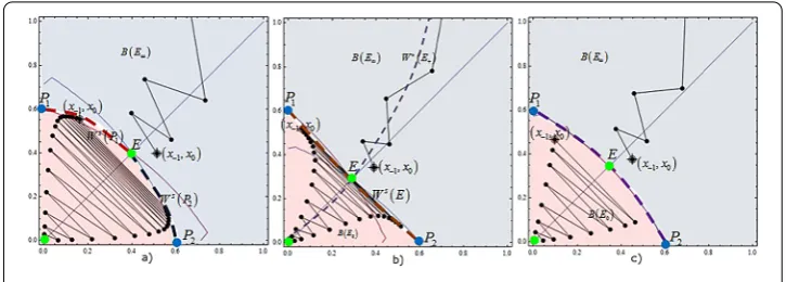
Figure 1 Visual illustration of Theorems 15 and 16.
(a)If B=D,F<G or B>D,F=G,then the positive equilibrium x+ is a repeller and
there exists the period-two solution which is a saddle point.In this case there exist four continuous curvesWs(P),Ws(P),Wu(P),andWu(P),with P= (,)and P= (,),
whereWs(P
)andWs(P)are passing through the point E+= (x¯+,x¯+)and they are graphs of
decreasing functions.The curvesWu(P
)andWu(P)are the graphs of increasing functions
which are starting at E(, ).Every solution{xn}which starts belowWs(P)∪Ws(P)in the
North-East ordering converges to Eand every solution{xn}which starts aboveWs(P)∪
Ws(P
)in the North-East ordering satisfieslimn→∞xn=∞. (See Figure(a).)
(b)If B=D,F>G or B>D,F=G,then the positive equilibrium x+is a saddle point and
there exists the period-two solution which is a repeller.Global behavior of()is described by Theoremwhere we set E(, )and E(x+,x+). (See Figure(b).)
(c)If B=D and F=G,then every point on the curve(),which is passing through the equilibrium E= (x¯+,x¯+),is a period-two solution of()except point E.Period-two
solu-tions and the positive equilibrium x+are nonhyperbolic points,while the zero equilibrium
is locally stable.The curve()divides the first quadrant into two regions.The region below ()in the first quadrant is a basin of attraction of the zero equilibrium and the region above the()in the first quadrant is a basin of attraction of point at infinity. (See Figure(c).)
Proof
(a) The existence of four curvesWs(P
),Ws(P),Wu(P), andWu(P) with the described
properties is guaranteed by Theorems and of [] applied to the mapTgiven by ().
The global result follows from Theorem .
(b) All conditions of Theorem are satisfied, which implies the proof.
(c) It was already noticed that every point on the curve () is a nonhyperbolic period-two solution of () and points
,–F+
F+ B( –I)
B
,
–F+F+ B( –I)
B ,
are the endpoints of () in the first quadrant. It is also known that the positive equilibrium x+is a nonhyperbolic point. This implies that the curve () which is passing through the
the basin of attraction of the points at infinity, it is a Julia set. LetVdenote the matrix
quadratic curves, we obtain the following statements:
• ifdetV> ⇔B>C, thenUis either an ellipse or a circle ifC= , • ifdetV< ⇔B<C, thenUis a hyperbole,
• ifdetV= ⇔B=C, thenUis union of two parallel lines.
We avoid the cases whenU is one point set or empty set. As a consequence ofI< and the fact that the curve () has endpoints in the first quadrant we conclude that the point (, ) is always below the curve (). It remains to describe global behavior of () when B=DandF=G. If an initial point (x–,x) is below the curve (), then
Now the proof is very similar and will be omitted. In this case both of the subsequences {xn}and{xn+}are increasing, which impliesxn→ ∞andxn+→ ∞.
If B=C, then
SinceF+ B( –I) > ,Uis the union of two parallel lines. If we want to obtain two
inter-secting lines it has to be B<Cand a straightforward calculation gives another condition F+ (B+C)( –I) = , which is not true.
.. The case:A=D=E=H=J= and I<
IfA=D=E=H=J= andI< , then (,) = (,–GI) is the period-two solution of the difference equation
xn+=Bxnxn–+Cxnxn–+Fxnxn–+Gxn–+Ixn–, ()
and the period-two solution (,) satisfies the system
=B+C+F+G+I, =B+C+F+G+I.
AsH+I< , there are locally stable zero equilibrium and positive unstable equilibrium. If B= andF=Gwe obtain the special case where (,) is the solution of the equation
C+F(+) +I– = .
Thus every point on the curveCxy+F(x+y) +I– = is a period-two solution of () except the equilibrium point (x+,x+).
One can see that in this case we obtain
a=B+F+I, b= , c=C+F, d= G+I.
Now,
(a– )(d– ) =B+F+I– (G+I– ) =B+F+I– ( –I), ad=B+F+I(G+I) =B+F+I( –I),
and
S–D– = –(a– )(d– ) = –B+F+I– ( –I).
Therefore,
B+F+I– = –I G
B( –I) +G(F–G), and for the positive equilibriumx+we have
q–p– = (C–B)x++ Gx++I–
= (C +B)x++ (F+G)x++I– =
– Bx++ (G–F)x+
• IfB( –I) +G(F–G) > , thenS–D– < ,D> –I> , and the period-two solution(,) = (,–GI)is a repeller. For example, ifF>G,B≥orF=G,eB> , thenq–p– < and the positive equilibriumx+is a saddle point.
• IfB( –I) +G(F–G) = , thenS–D– = and the period-two solution
(,) = (,–GI)is a nonhyperbolic point. For example ifF=GandB= , then the positive equilibriumx+is a nonhyperbolic point and every point on the curve
Cxy+F(x+y) +I– = is a period-two solution of (), except(x+,x+). The points
(,) ={(,–GI), (–GI, )}are the endpoints of the curveCxy+F(x+y) +I– = in the first quadrant.
• IfB( –I) +G(F–G) < , thenS–D– > and the period-two solution
(,) = (,–GI)is a saddle point andB( –I) +G(F–G) < . For example ifF<Gand B= , thenq–p– > and the positive equilibriumx+is repeller.
One can prove that in this case the mapT has no other minimal period-two solutions
except (,) = (,–G+ √
G+D(–I)
D ). This leads to the following theorem.
Theorem Let A=D=E=H=J= and I< ,then()has locally stable zero equilib-rium and the positive equilibequilib-rium x+.The following statements hold:
(a)If B= and F<G,then the positive equilibrium x+ is repeller and there exists the
period-two solution which is a saddle point.In this case there exist four continuous curves Ws(P
),Ws(P),Wu(P),andWu(P).The curvesWs(P)andWs(P)are passing through
the point E+= (x¯+,x¯+)and they are graphs of decreasing functions.The curvesWu(P)and
Wu(P
)are the graphs of increasing functions and are starting at E(, ).Every solution
{xn}which starts belowWs(P
)∪Ws(P)in the North-East ordering converges to Eand
every solution{xn}which starts aboveWs(P
)∪Ws(P)in the North-East ordering satisfies
limn→∞xn=∞. (See Figure(a).)
(b)If F>G,B≥or F=G,B> ,then the positive equilibrium x+is a saddle point and
there exists the period-two solution which is repeller.Global behavior of()is described by Theoremwhere we set E(, )and E(x+,x+). (See Figure(b).)
(c)If F=G and B= ,then every point on the curveJ=Cxy+F(x+y) +I= ,which is
passing through the point E= (x¯+,x¯+),is a period-two solution of()except E.All
period-two solutions and the positive equilibrium x+are nonhyperbolic points and the zero
equi-librium is locally stable.The curveJdivides the first quadrant into two regions.The
re-gion belowJin the first quadrant is the basin of attraction of the zero equilibrium and
the region aboveJin the first quadrant is the basin of attraction of point at infinity. (See
Figure(c).)
Proof
(a) The existence of four curvesWs(P),Ws(P),Wu(P), andWu(P) with the described
properties is guaranteed by Theorems and of [] applied to the mapTgiven by ().
The global result follows from Theorem .
(b) All conditions of Theorem are satisfied and the proof follows from Theorem . (c) The facts that every point on the curveJis a nonhyperbolic period-two solution of
(), except (x+,x+), and that the points (,) ={(,–GI), (–GI, )}are the endpoints ofJ
in the first quadrant were proven earlier. This implies that the curveJ, which is passing
through the pointE= (x¯+,x¯+) is not a global stable manifold ofE. It remains to describe
the first quadrant, the point (, ) is always below the curve. If the point (x–,x) is below
the Julia setJ, then
Cx–x+F(x–+x) +I< .
Asxn+= (Cxnxn–+F(xn+xn–) +I)xn–, we have
x=
Cxx–+F(x+x–) +I
x–<x–,
x=
Cxx+F(x+x) +I
x<
Cxx–+F(x+x–) +I
x<x.
Thus the point (x,x) is belowJtoo and
Cxx+F(x+x) +I< .
Now
x=
Cxx+F(x+x) +I
x<x,
x=
Cxx+F(x+x) +I
x<
Cxx+F(x+x) +I
x<x.
Continuing in this way, we obtain (, )ne· · · ne(x,x)ne(x,x)ne(x–,x). Hence,
both subsequences{xn}and{xn+}are decreasing, which impliesxn→ andxn+→.
If we start at the point (x–,x) aboveJ, then
Cx–x+F(x–+x) +I> ,
which, in a similar way as above implies (x–,x)ne(x,x)ne. . . . In this case both
sub-sequences{xn}and{xn+}are increasing, which implies thatxn→ ∞andxn+→ ∞.
The special cases studied in Theorem leads to the following general result.
Theorem Consider the difference equation
xn+=P(xn,xn–)xn–, ()
where P is a symmetric polynomial function with nonnegative coefficients.If we assume that P(, ) < ,then the curve P(x,y) = is the Julia set and separates the first quadrant into two regions:the region below the curve is the basin of attraction of E(, )and the
region above the curve is the basin of attraction of a point at infinity.
Proof Equilibrium points of () are solutions of the equation
x=P(x,x)x ⇔ xP(x,x) – = ,
which implies that () has zero equilibrium. Leth(x) =P(x,x) – . Then
and we see that the equationP(x,x) = has exactly one positive equilibriumx+. As a
con-sequence of the symmetry we have ∂P
∂x(x,y) =
∂P
∂y(y,x) and
p+q=x
∂P ∂x(x,x) +
∂P ∂y(x,x)
+P(x,x)
= x∂P
∂x(x,x) +P(x,x),
wherepandqdenote partial derivatives of functiong(x,y) =yP(x,y) evaluated at the equi-libriumx. For the zero equilibrium we get
p+q=P(, ) < ,
and by applying Proposition , the zero equilibrium is locally asymptotically stable. Simi-larly, in the case of the positive equilibriumx+, we get
p+q= x+
∂P
∂x(x+,x+) +P(x+,x+)
= x+
∂P
∂x(x+,x+) + ≥
and
q–p=P(x+,x+) = .
By applying Proposition the positive equilibriumx+is unstable nonhyperbolic point.
The period-two solution{,}, where ≤<, satisfies the system
=P(,),
=P(,).
Since> , we haveP(,) = andP(,) =P(,) = . Hence, every point of the setJ={(x,y) :P(x,y) = }is a period-two solution of () except the equilibrium point
(x+,x+). If we start at the point (x,x–) below the curveJ, then
P(x,x–) <
and from the fact thatP(x,y) is an increasing function in both variables we obtain the following:
x=P(x,x–)x–<x–,
x=P(x,x)x<P(x–,x)x=P(x,x–)x<x.
Therefore the point (x,x) is also belowJand
So
x=P(x,x)x<x,
x=P(x,x)x<P(x,x)x=P(x,x)x<x.
Continuing in this way, we obtain (, )ne· · · ne(x,x)ne(x,x)ne(x–,x). Hence,
both subsequences{xn}and{xn+}are decreasing, which impliesxn→ andxn+→.
If we start at the point (x–,x) aboveJ, then
P(x,x–) > .
The proof of the remaining case is similar and will be omitted. In this case both subse-quences{xn}and{xn+}are increasing, which impliesxn→ ∞andxn+→ ∞.
.. The Case:J= ,H+I≥
Next we consider the case where J= andH+I≥. In this case () has exactly one equilibrium which is the zero equilibrium, which in view of Proposition is unstable.
The following result describes a global dynamics of () in this case.
Theorem Consider()under the conditions J= and H+I≥.The global behavior of solutions of()is as follows:
(a) If –H<I≤and()does not possess a period-two solution,then every solution
{xn}of()satisfieslimn→∞xn=∞;
(b) If –H=I≤,then every solution{xn}of()is either a period-two solution or it satisfieslimn→∞xn=∞;
(c) If +H<Iand()does not possess a period-two solution,then every solution{xn}of
()satisfieslimn→∞xn=∞.
Proof
(a) In view of Theorem there exist the global stable manifoldWs(, ) and the global unstable manifoldWu(, ), whereWs(, ) is a graph of continuous decreasing curve and Wu(, ) is a graph of continuous increasing curve and both manifolds are invariant sets. The only decreasing curve in the first quadrantQpassing through (, ) is the union of
the coordinate axes, but this set is clearly not an invariant set, which means thatWs(, ) is not a part ofQ. On the other handWu(, ) exists and all solutions are asymptotic to
Wu(, ). Thus if () does not possess a period-two solution, then every solution{xn}of () satisfieslimn→∞xn=∞.
(b) Assume that{xn}is not a minimal period-two solution of (). Then{xn}is eventually monotone or the subsequences{xn}and{xn+}are eventually monotone. If{xn}is
even-tually decreasing, thenxn<xn–for alln≥K, which impliesxn+≥Hxn+Ixn–> (H+I)xn= xn, which is a contradiction. If the subsequences{xn}and{xn+}are eventually
mono-tone, then without loss of generality we can assume that{xn}is eventually nondecreasing
and{xn+}is eventually non-increasing. In this casexn→ ∞, which would imply that xn+→ ∞, which is a contradiction. Thus the remaining possibility is that{xn}is
To complete this we will find the image ofE+tv, wheret> and v is the eigenvector that corresponds to the eigenvalue , under the mapT. SinceE+tv= (t,t), we have
T(E+tv) – (E+tv) =T(t,t)– (t,t) =, (A+B+C+D)t+ (E+F+G)t+ (H+I– )t. By using the conditionH+I– = , we have
T(E+tv) – (E+tv) =, (A+B+C+D)t+ (E+F+G)t,
which impliesE+tvneT(E+tv) for everyt> . This shows that every point in u∈(x,¯ ∞)
is a supersolution for the mapT, that is, uneT(u), see [], and so every solution tends to∞.
(c) In view of I> +H from () we havexn+ >Ixn–, which implies xn+>Ikx– or
xn+>Ikx for somek such thatk→ ∞asn→ ∞. Consequently every solution {xn}
of () satisfieslimn→∞xn=∞.
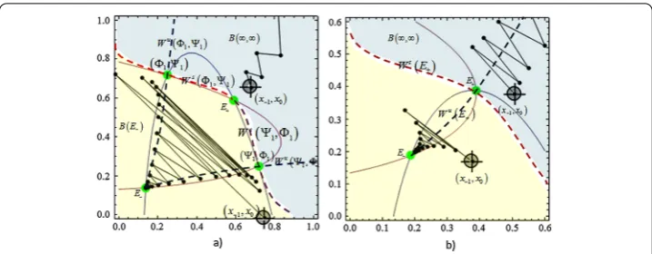
4.2 The case of two equilibrium points and a finite number of hyperbolic minimal period-two solutions
In this section we present the global dynamics of () in the parametric regions where there exist two distinct equilibrium pointsE–(x¯–,x¯–) andE+(x¯+,x¯+), such thatE–neE+, which
holds if and only if
S(S– SS) –
(S
– SS)
S
+J< ,
and a finite number of period-two solutions which are hyperbolic. In this case, we prove that the Julia set is the union of the stable manifolds of some saddle period-two points and separates the first quadrant into two regions: the region below the curve is the basin of attraction ofE– and the region above the curve is the basin of attraction of the point at
infinity.
Let T(x,y) = (g(x,y),h(x,y)) whereg(x,y) =f(y,x) and h(x,y) =f(f(y,x),y). Then the
period-two curves, that is, the curves of which the intersection is a period-two solution, are given by
CF˜:=
(x,y) :f(y,x) =x=(x,y) :g(x,y) =x and CG˜ :=
(x,y) :f(x,y) =y=(x,y) :h(x,y) =y. Let
˜
F(x,y) :=Dx+ (Cy+G)x+By+Fy+I– x+Ay+Ey+Hy+J, ˜
G(x,y) :=Ax+ (By+E)x+Cy+Fy+Hx+Dy+Gy+ (I– )y+J, P(y) := (A+B+C+D)y+ (E+F+G)y+ (H+I– )y+J.
The following lemma gives some properties ofF(x,˜ y),G(x,˜ y),Resx(F,˜ G), and˜ Resy(F,˜ G).˜
Lemma The following hold:
(i) F(x,˜ y) =G(y,˜ x)anddegx(F) =˜ degy(G)˜ ≤,anddegy(F) =˜ degx(G)˜ ≤,where the indices indicate in which variable we consider that polynomial.
(ii) Ifs(y) =Resx(F,˜ G)˜ andr(x) =Resy(F,˜ G),˜ thenr(x) = (–)degx(F˜)·degx(G˜)s(x).
Proof
(i) The proof follows from the factF(x,˜ y) =f(y,x) –xandG(x,˜ y) =f(x,y) –y. (ii) LetF(x,˜ y) :=i=ai(y)xiandG(x,˜ y) :=
i=bi(y)xi. SinceF(x,˜ y) =G(y,˜ x), we obtainF(x,˜ y) :=i=bi(x)yiandG(x,˜ y) :=
i=ai(x)yi. From this and the definition of the Sylvester matrix we getr(x) = (–)degx(F˜)·degx(G˜)s(x).
LetPi,i= , , , be the polynomials in the Appendix. The following lemma gives us information as regards the number of minimal period-two solutions.
Lemma Assume thatResx(F,˜ G) =˜ P(y)P(y)≡.Then there exist at mostdeg(P)/
isolated minimal period-two solutions. Let PS denote the number of isolated minimal period-two solution.The following statements are true:
(i) IfA> andD> ,thenResx(F,˜ G) = –P˜ (y)P(y).IfP≡,then PS≤.
(ii) IfA= andD> ,thenResx(F,˜ G) = –D˜ –degx(G˜)P(y)P(y).IfP≡,then PS≤.
(iii) IfD= andA> ,thenResx(F,˜ G) = (–)˜ degx(F˜)A–degx(F˜)P(y)P(y).IfP≡,then
PS≤.
(iv) IfA=D= ,C+B> ,C+G> ,andB+E> ,thenResx(F,˜ G) =˜ P(y)P(y).If
P≡,then PS≤.
(v) IfA=D= ,B=E= ,andC> ,thenResx(F,˜ G) =˜ P(y)P(y).IfP≡,then
PS≤.
(vi) IfA=D= ,C=G= ,andB> ,thenResx(F,˜ G) =˜ P(y)P(y).IfP≡,then
PS≤.
Proof Suppose that{,}is a minimal period-two solution (=). ThenF(,˜ ) = ˜
G(,) = , Lemma , and Theorem implyResx(F,˜ G)() =˜ Resy(F,˜ G)() = , and we˜ see thatP() =P() = . This implies that there exist at mostdeg(P)/isolated minimal period-two solutions. By using the packageMathematica, one can see that the statements
(i)-(vi) are true.
The following lemma gives the necessary conditions under which an isolated period-two solution is nonhyperbolic.
Lemma Assume thatResx(F,˜ G) =˜ P(y)P(y)≡ (i.e. P(y)≡).Then the following
state-ments hold:
(i) If ()has a nonhyperbolic period-two solution,thenDis(P) = . (ii) If ()has a nonhyperbolic equilibrium point,then
Dis(P·P) =Dis(P)Dis(P)Res(P,P)= ,