University of South Carolina
Scholar Commons
Theses and Dissertations
12-14-2015
Numerical and Experimental Investigations of Dam
and Levee Failure
Ezzat Youssef Elhassan Mohamed Elalfy
University of South Carolina - ColumbiaFollow this and additional works at:https://scholarcommons.sc.edu/etd Part of theCivil Engineering Commons
This Open Access Dissertation is brought to you by Scholar Commons. It has been accepted for inclusion in Theses and Dissertations by an authorized administrator of Scholar Commons. For more information, please [email protected].
Recommended Citation
Numerical and experimental investigations of dam and levee failure
by
Ezzat Youssef Elhassan Mohamed Elalfy
Bachelor of Science Ain Shams University, 2004
Master of Science Ain Shams University, 2008
Submitted in Partial Fulfillment of the Requirements
for the Degree of Doctor of Philosophy in
Civil Engineering
College of Engineering and Computing
University of South Carolina
2015
Accepted by:
M. Hanif Chaudhry, Major Professor
Jasim Imran, Committee Member
Enrica Viparelli, Committee Member
Jamil Khan, Committee Member
Dedication
Acknowledgments
I would like to thank my dissertation advisor, Prof. M. Hanif Chaudhry for his
sup-port, and continuous encouragement; his door was always open to address research
problems. Thanks are also extended to my dissertation committee members: Prof.
Jasim Imran and Dr. Enrica Viparelli for their continuous advice and invaluable
suggestions during our weekly group meetings. Also, thanks are extended to my
dis-sertation committee member Prof. Jamil Khan for the time he devoted for reviewing
my manuscript.
Thanks are extended to my former and current colleagues in the water resources
group: Dr. Khaled Abdo, Dr. Cyrus K. Riahi-Nezhad, Dr. Lindsey LaRocque, Dr.
Mohamed Elkholy, Ali Asghari Tabrizi, and Hassan Ismail for continuously sharing
ideas. Many thanks to Paul Sagona from the Research Cyberinfrastructure of the
University of South Carolina for training me on how to run my codes on the
super-computer.
Special thanks to the Egyptian Cultural and Educational Bureau for supporting me
during the course of my study. Also, the funding from the National Science
Founda-tion under the PIRE program, Grant No. OISE 0730246 is gratefully acknowledged.
No words can describe my deep gratitude to my father, mother, sisters, and brother
for their continuous moral support during my study. Also, my sincere appreciation
to my wife and my kids for their prayers and supplications to Allah to help me pass
Abstract
Both numerical and experimental investigations are conducted to study the failure of
earthen dams and levees.
Boussinesq equations describing one-dimensional unsteady flow including
non-hydros-tatic pressure distribution are solved numerically along with Exner equation for the
sediment mass conservation to include the effects of the streamline curvature on the
failure of non-cohesive earthen embankments. In addition, the effects of the steep
bottom slope on the flow variables during the failure are studied by solving the
Saint-Venant equations modified for steep bed slope along with the Exner equation to
simulate non-cohesive earthen embankment failure due to overtopping. The
Boussi-nesq equations are solved by using the two-four finite-difference scheme which is
second order accurate in time and fourth order accurate in space, while the modified
Saint-Venant equations are solved by using the MacCormack finite-difference scheme
which is second order accurate in time and space. The performance of three
sedi-ment transport formulae, namely Ashida and Michiue, Meyer-Peter and Müller, and
Modified Meyer-Peter and Müller for steep slope is compared. The comparison of the
numerical results with the experimental results shows that: (1) The improvement in
the prediction of the breach evolution and the downstream hydrograph by including
the Boussinesq terms is minimal; (2) The predicted results by using the modified
Saint-Venant equations are slightly better than those calculated by using the
classi-cal Saint-Venant equations; (3) Ashida and Michiue transport equation overestimates
the erosion rate which results in an overestimation of peak discharge but predicts the
Müller equations give almost the same results for the top elevation of the eroded dam
and the water surface levels, and the peak value and time to peak of the downstream
hydrograph. A number of non-dimensional equations are presented to relate different
model variables to the peak discharge of the downstream hydrograph. A sensitivity
analysis of different model parameters to determine the most dominant factor
affect-ing the peak downstream discharge indicates that the most dominant factor affectaffect-ing
the peak discharge is the upstream reservoir volume, while the sediment grain size
shows very little effect on the peak discharge.
The lateral outflow through a levee breach may be computed as an outflow over a
broad-crested side weir. The lateral outflow has been computed previously by
assum-ing the flow in the main channel to be one-dimensional, and most of the equations for
computing the outflow are based on the local flow variables near the breach. These are
unknown and difficult to measure during a flood. In this study, a numerical model is
developed to solve the two-dimensional, shallow water equations using MacCormack
finite-difference scheme. The model is applied to a breach in a rectangular channel.
A comparison of the numerical results with the experimental measurements shows
satisfactory agreement. Different cases are simulated by varying the breach width,
the bottom level of the breach, and the discharge in the main channel. Comparison
between the breach outflows obtained using the numerical model with the results of
a simple one-dimensional approach indicates that the breach outflows are
overesti-mated by the latter. A new discharge correction factor is introduced for the lateral
breach outflow predicted using the simple one-dimensional approach. The correction
factor is a function of the submergence ratio of the breach, breach width, and inlet
Froude number.
An accurate prediction of the evolution of the breach resulting from overtopping
of a non-cohesive earthen levee is important for flood mitigation studies.
depths. The breach shape is recorded using a sliding rods technique. A sequence of
discrete mass failure of the sides of the breach due to slope instability is observed
dur-ing the failure process. A simple geostatic failure mechanism is suggested to calculate
the lateral sediment load due to the mass failure. This mechanism is implemented in
a two-dimensional numerical model which solves the shallow water equations along
with the sediment mass conservation. In order to assess the effect of the lateral
sedi-ment load resulting from slope instability on the failure process, the predicted breach
shape evolution and breach hydrograph with and without the slope failure mechanism
are compared with the experimental results. The predicted breach shape is improved
by adding the lateral sediment inflow due to slope instability especially in terms of
the maximum depth of erosion. Also, the peak discharge of the breach hydrograph is
Table of Contents
Dedication . . . ii
Acknowledgments . . . iii
Abstract . . . iv
List of Tables . . . x
List of Figures . . . xi
Chapter 1 Introduction . . . 1
1.1 General . . . 1
1.2 Objectives and scope of the study . . . 2
Chapter 2 Literature review . . . 3
2.1 Earthen dam failure . . . 3
2.2 Steady flow through breached levees . . . 6
2.3 Gradual failure of earthen levees . . . 7
2.4 Conclusions . . . 9
3.1 Introduction . . . 11
3.2 Experimental setup . . . 11
3.3 Numerical model description . . . 13
3.4 Model application . . . 21
3.5 Summary and conclusions . . . 23
Chapter 4 Estimation of Outflow Discharge Through Differ-ent Levee Breach Sizes Using One- and Two-Dimensional Models . . . 38
4.1 Introduction . . . 38
4.2 Experimental setup . . . 39
4.3 Numerical model description and solution procedure . . . 39
4.4 Model application . . . 44
4.5 Summary and conclusions . . . 48
Chapter 5 Numerical and Experimental Investigations on Ge-omorphic Levee Breach Including Geostatic Fail-ure Mechanism . . . 64
5.1 Introduction . . . 64
5.2 Experimental setup . . . 65
5.3 Numerical model description . . . 66
5.4 Model application . . . 69
5.5 Summary and conclusions . . . 70
Chapter 6 Summary and Conclusions . . . 90
6.2 Recommendations for future investigations . . . 92
List of Tables
Table 4.1 Range of model variables . . . 50
List of Figures
Figure 3.1 Experimental setup (all dimensions are in meters) . . . 25
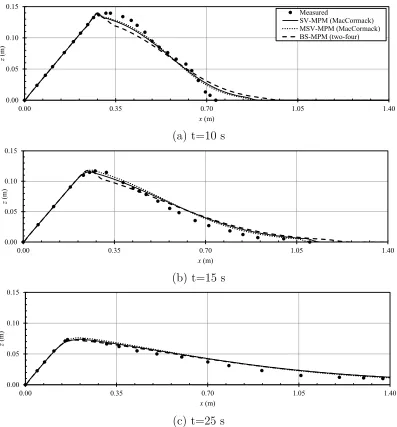
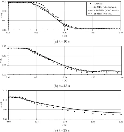
Figure 3.2 Dam surface at various times using different numerical models . . 27
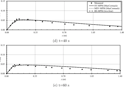
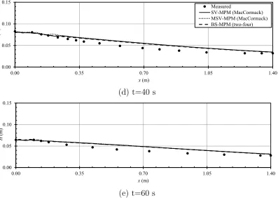
Figure 3.3 Water surface at various times using different numerical models . 29
Figure 3.4 Downstream hydrograph using different numerical models . . . . 30
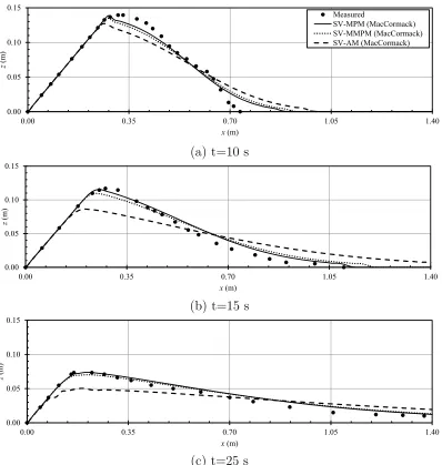
Figure 3.5 Dam surface at various times using different sediment transport
formulae . . . 32
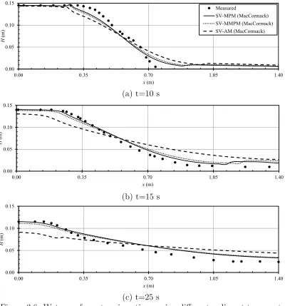
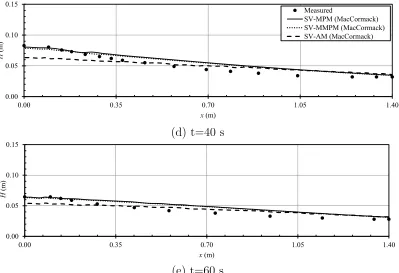
Figure 3.6 Water surface at various times using different sediment
trans-port formulae . . . 34
Figure 3.7 Downstream hydrograph using different sediment transport formulae 35
Figure 3.8 Effect of embankment top width on the peak discharge . . . 36
Figure 3.9 Effect of reservoir volume on the peak discharge . . . 36
Figure 3.10 Effect of inlet discharge on the peak discharge . . . 36
Figure 3.11 Effect of percentage change of the variable on the peak discharge 37
Figure 4.1 Experimental model of a levee breach of a rectangular channel
(Riahi-Nezhad, 2013) (not to scale, all dimensions in meters) . . . 51
Figure 4.2 Comparison between numerical (dashed line) and measured (dots)
results . . . 54
Figure 4.3 Flow variables across the main channel at the breach upstream
section forSr and bb = 0.73, 1.6 m, respectively . . . 55
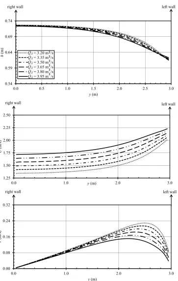
Figure 4.4 Flow variables across the main channel at the breach upstream
Figure 4.5 Effect ofSr onh/hd.s and qb/qi for (Qi = 3.2m3/s and bb = 1.6 m) 57
Figure 4.6 Effect ofbr on h/hd.s and qb/qi for (Qi = 3.2 m3/s andSr = 0.6) . 58
Figure 4.7 Normalized Qb for different cases . . . 60
Figure 4.8 cr for different cases . . . 62
Figure 4.9 cr(fitted equation) vs cr(simulated) . . . 63
Figure 5.1 Experimental model of fully developed levee breach (not to
scale, all dimensions in meters) . . . 73
Figure 5.2 Experimental model with earthen levee (not to scale, all
dimen-sions in meters) . . . 74
Figure 5.3 Geostatic failure mechanism . . . 75
Figure 5.4 Solution procedure . . . 76
Figure 5.5 Comparison between numerical and measured water depth . . . . 80
Figure 5.6 Comparison between numerical and measured surface velocity . . 82
Figure 5.7 Comparison between numerical and measured breach shape
(scenarios 1,2,3) . . . 85
Figure 5.8 Comparison between numerical and measured breach shape(scenarios 4,5) . . . 88
Figure 5.9 Maximum breach depth with time(scenarios 1,2,3,4,5) . . . 88
Chapter 1
Introduction
1.1 General
Dams and levees, also known as embankments, are structures used for water
stor-age, water level regulation in streams, recreation activities, power generation, and for
the protection of surrounding areas against floods. Failure of these structures may
result in catastrophic property damage and loss of life. In the last few decades, the
climate has changed significantly due to Global Warming which leads to ice melt,
and sea level rise. This has increased the intensity and frequency of heavy storms
such as hurricanes Katrina (2005), Sandy (2012), and Joaquin (2015). Embankments
may be classified according to the material of construction as non-erodible, such as
concrete, and erodible, such as earth and rock fill. The latter type is more
prefer-able for construction due to the availability of material and the low construction
costs. Failure of concrete dams usually happens suddenly when part of the structure
is overstressed. However the failure of an earthen embankment is gradual, and the
simulation of the flow field is more complex. This requires an appropriate
under-stating of the interaction between the water and the soil. Almost 80 percent of the
dams in the United States are constructed from erodible material (U.S. Committee
on Large Dams, 1975). The major causes of the failure of earthen embankment are:
overtopping, structural defects, and piping. The present study only focuses on the
1.2 Objectives and scope of the study
The main objectives of this research are to develop one- and two-dimensional
nu-merical models to accurately predict the breaching process of earthen embankments
and the resulting hydrograph. In order to develop these numerical models, the
fol-lowing tasks are proposed:
1- Conduct small scale experiments on earthen embankment failure due to plane
surface erosion, and use the measured results for numerical model validation.
2- Develop a one-dimensional numerical model based on the classical, shallow-water
equations with sediment mass conservation.
3- Investigate the effect of steep slope on the pressure, gravity, and friction terms of
the shallow-water equations.
4- Investigate the effect of non-hydrostatic pressure assumption on the shallow-water
equations.
5- Develop and validate a two-dimensional numerical model to simulate the steady
state flow field due to levee breach in rectangular and trapezoidal channels.
6- Develop a two-dimensional numerical model including slope failure mechanism to
simulate the gradual failure of a non-cohesive earthen levee.
In the present study, the literature is reviewed in Chapter 2. Different governing
equations with various sediment transport formulations to simulate one-dimensional
plane embankment failure are presented in Chapter 3. Chapter 4 discusses the
esti-mation of the steady outflow discharge through levee breach of a rectangular channel
using one- and two-dimensional numerical models. Two-dimensional numerical
mod-eling of gradual failure of earthen levee including slope failure mechanism is presented
in Chapter 5. Finally, the summary and conclusions of these studies are presented in
Chapter 2
Literature review
2.1 Earthen dam failure
Dams are barriers constructed across streams for water storage, irrigation, navigation,
flood control, power generation, and recreation activities. About 58 percent of the
dams in the world are earthen embankments and the remainder are made of concrete
(Costa, 1985). This may be due to their low construction costs, availability of
con-struction materials, and no special foundation requirements. Earthen embankments,
the oldest type of dams, are generally the most economical and have a spillway to
control the upstream water level. According to the Fourth Inter-governmental
Cli-mate Change Assessment (IPCC, 2013), the intensity and the frequency of occurrence
of heavy storms has increased in the last two decades, which may lead to flood events
that exceed the design capacity of embankment spillways, thereby causing
overtop-ping and failure. In the United States about 57,000 dams have the potential for
overtopping (Ralston, 1987). An accurate prediction of peak discharge and time to
peak in case there is an embankment breach is needed for preparing emergency action
plans and risk assessments.
The major causes of earthen embankment failure may be classified into three
cate-gories (ASCE/EWRI Task Committee on Dam/Levee Breaching, 2011): Overtopping
(34%), piping (28%) and structural failure (30%). If a dam is overtopped, the water
embank-ment surface when the hydraulic shear stress exceeds the critical shear stress of the
soil. Piping or internal erosion occurs when fine materials between upstream and
downstream slope are washed by seepage and a pipe is formed inside the
embank-ment. The diameter of this pipe increases with time due to an increase in the internal
discharge until the embankment collapses internally. Structural failure includes slope
instability, differential settlement, and sliding. The present work focuses only on the
overtopping failure.
The past research may be classified into two major categories: (1)
Experimen-tal investigations and (2) Numerical modeling. These are discussed in the following
paragraphs.
Experimental investigations
Tinney and Hsu (1961) conducted experiments on the mechanics of washout of fuse
plugs utilizing the sediment transport equations. Simmler and Samet (1982)
inves-tigated the evolution of embankment erosion due to overtopping. They found that
the erosion process is affected by the dam material, dam geometry, reservoir
vol-ume, and the location of impervious element. They also provide a relationship for
the breach flow as a function of the breach volume. Coleman et al. (2002) studied
the failure of non-cohesive homogenous embankments due to overtopping along the
crest of the embankment. They derived expressions to predict the development of
the breach shape, eroded volume, and breach flows. Dupont et al. (2007) carried
out a scale-model study to validate a numerical model for the time evolution of dam
breach and the outflow hydrograph. Schmocker and Hager (2009) carried out a series
of experiments of plane embankment breach of loose, uniform, non-cohesive sediment
to study the test repeatability, side-wall, and scale effects. Pickert et al. (2011)
breach discharge, breach profile, erosion rates, and pore-water pressure within the
embankment.
Numerical modeling
Wang and Bowles (2006a,b) presented a slope stability model with a finite-difference
scheme to simulate the dam-breach outflow by solving the two-dimensional
Saint-Venant equations. They applied their numerical model to an arbitrary breach in a
non-cohesive earthen embankment due to overtopping failure. Pontillo et al. (2010)
applied a two-phase, one-dimensional numerical model based on the shallow water
equations coupled with a sediment erosion model for the case of loose, non-cohesive,
homogenous, earthen embankment. Their numerical results reasonably match the
measured temporal free surface and bed evolution of the experimental data. They
indicate some inaccuracies in the numerical results due to streamline curvature.
Van Emelen et al. (2011) developed two numerical models; the first model is based on
the classical two-dimensional Saint-Venant equations coupled with the Exner
equa-tion with a Meyer-Peter and Müller formula for calculating the sediment transport
rate; and the second model includes a two-dimensional bank failure mechanism into
the classical, two-dimensional shallow-water model. Both models assume hydrostatic
pressure and neglect the effects of streamline curvature. Van Emelen et al. (2012)
applied two numerical approaches involving different sediment transport formulae for
solving the breach in a channel with a loose, non-cohesive sand embankment due to
overtopping. The first model utilized coupled Saint-Venant-Exner equations, and the
second model assumes a mixture layer of water and sediment. They concluded that
2.2 Steady flow through breached levees
A levee is a structure, constructed by humans or formed naturally along the course of a
river to regulate its water level and or to protect its floodplain. Due to climate change,
the risk has increased of large scale disasters caused by levee breach (Kakinuma and
Shimizu, 2014). The assessment of this risk requires the identification of various
geometric and hydraulic parameters causing this failure.
Several levee breaches occurred in the last decade: New Orleans, Louisiana 2005,
Fernley, Nevada burst 2008, Munster, Indiana 2008, Southern Taiwan 2009, Vendée,
France 2010, and Poplar Bluff, Missouri 2011. The death and property damage
caused by these events was greater than the failure of any other man-made structure,
especially because most of these levees were constructed near urban areas.
Levee breach has been studied by several researchers. Jaffe and Sanders (2001)
developed a model for flood mitigation by designing an engineered levee breach which
creates depression waves that interact with the flood wave to reduce the flood stages at
certain locations of the channel where severe damage from flooding would be expected.
Their model is based on the solution of the two-dimensional shallow water equations
by finite-volume method. They derived a non-dimensional relation to calculate the
optimal flood plain area of the engineered levee breach. Sattar et al. (2008) tested
a 1:50 scale model of the 17th street canal breach in New Orleans based on Froude
similitude relationships. They investigated different procedures for breach closure.
Han et al. (1998) developed a combined, one- and two-dimensional hydrodynamic
model. The one-dimensional model is based on the dynamic wave equation and
utilizes Preissmann scheme which is an implicit, finite-difference method. The
two-dimensional model solves a diffusion wave equation by integrated finite differences.
They applied their model to an actual levee-break in the downstream reaches of the
Han river. They validated the simulated results with the observed data, including
conducted a physical model of an urban district and provided water depth history of
different configurations of the model city for the purpose of mathematical modeling.
Soares-Frazão et al. (2008) introduced a two-dimensional, shallow-water model with
porosity for urban flood modeling and solved the governing equations by finite volume
method. They compared their results with experimental measurements. Their model
reproduced the mean characteristics of the flow inside and around the urban area
with low computational cost compared to the classical shallow-water model.
Roger et al. (2009) solved the shallow-water equations by using a total variation
diminishing, Runge-Kutta discontinuous Galerkin finite-element method, and by
us-ing a finite-volume scheme involvus-ing a flux vector splittus-ing approach. Both models
had satisfactory agreement with the experimental results. They also found that the
simulated results are less sensitive to the bed and wall roughness and to the
turbu-lence modeling due to the advective nature of the levee-breach flow which is governed
mainly by the pressure gradient and the advective terms in the momentum equations
rather than the diffusion. Kesserwani et al. (2010) presented new governing equations
for predicting flow divisions at open-channel T-junctions. The new approach predicts
the lateral-to-upstream discharge for different flow regime satisfactorily. Van Emelen
et al. (2012) developed a finite-volume model to solve the two-dimensional,
shallow-water equations. The model was applied to an idealized case study of 17th street
canal breach in New Orleans, Louisiana. The steady-state numerical results
satisfac-torily agreed with the experimental results. They concluded that the depth-averaged
models give an acceptable flow prediction in the complex domains at reasonable
com-putational cost.
2.3 Gradual failure of earthen levees
According to the U.S. Committee on Large Dams (1975), about 80 percent of the
earthen levee failure process (i.e., breach shape evolution, breach hydrograph, and the
resulting flow field) is quite complex, requiring deep understanding of the interaction
between the water flow, sediment transport, and the corresponding geomorphological
changes.
The breaching process in dams and levees differs due to the direction of the
mo-mentum flux (ASCE/EWRI Task Committee on Dam/Levee Breaching, 2011). A
variety of research was conducted in the past concerning earthen embankment
breach-ing, however few of that research focused on the earthen levee failure.
Faeh (2007) developed a two-dimensional numerical model, 2bMb, which uses a
finite-volume approach to solve the shallow-water equations and a sediment transport
module for bed and suspended load for an arbitrary number of grain size classes. The
model was validated with the results of experiments of dam breaks due to erosion
(Bechteler and Kulisch, 1998), and field data of one of the dike breaches on the
Elbe River following a flood in Sachsen (Germany) 2002. He found that, the most
sensitive parameter of an earthen dike failure, is the breach side-slope which affects
the lateral erosion. Kakinuma and Shimizu (2014) conducted large-scale experiments
on riverine levee breach. They categorized the levee failure process into four stages:
(1) Downstream slope erosion; (2) The erosion advances to the top of the upstream
slope, and the breach at the crest starts to widen; (3) The breach widening advances
in the downstream direction and the breach outflow peaks; (4) The breach outflow
becomes constant and the rate of breach widening is decreased. They proposed
a breach rate equation similar to the sediment transport formula by Meyer-Peter
and Müller (1948) using their experimental measurements. The proposed equation
substituted the sediment transport formula for the levee cells in a two-dimensional
numerical model which solves the shallow-water equations. The numerical model was
validated using the experimental measurements and the breach widening stage was
failure.
2.4 Conclusions
Earthen dam failure
To the best of the author’s knowledge, all cited studies used the classical Saint-Venant
equations with the hydrostatic pressure assumption and neglected the steep slope
and streamline curvature effects on the erosion process. The objectives of the present
work are to study the effects of steep slope and streamline curvature on the failure of
non-cohesive earthen embankments by modifying the the governing equations for the
flow, assess the performance of various sediment transport formulas, and determine
the most dominant factor affecting the peak discharge of the downstream hydrograph.
Steady flow through breached levees
Most of the cited studies are for special cases of levee breach. In the present work,
a generalized approach is used to study levee breach by considering the lateral
out-flow through a levee breach as lateral outout-flow over a broad-crested side weir. Most
of the previous studies predicted the flow over a side weir by applying the energy
principle in the longitudinal direction and assume the flow in the main channel is
one-dimensional (Chow, 1959; Subramanya and Awasthy, 1972; Hager, 1987; Singh
et al., 1994; Swamee et al., 1994; Borghei et al., 1999). The objectives of the present
study are to develop a numerical model based on two-dimensional depth-averaged
equations to simulate the flow field resulting from a generalized levee breach of a
rectangular channel and to develop a non-dimensional equation to calculate the
dis-charge correction factor for the breach disdis-charge estimated using the one-dimensional
Gradual failure of earthen levees
The effects of the lateral sediment inflow on the failure shape evolution and on the
flood hydrograph of an earthen levees have not been studied. This lateral sediment
inflow is caused by the slope instability of breach sides. The objective of the present
study is to include this sediment inflow in a two-dimensional depth-averaged model
Chapter 3
Numerical and Experimental Investigations on
Earthen Embankment Breach due to
Overtopping
3.1 Introduction
The one-dimensional earthen embankment breach has been studied extensively during
the last few decades. However, most of these studies used the classical Saint-Venant
equations with the hydrostatic pressure assumption and neglected the effects of steep
slope and streamline curvature on the erosion process. The objectives of the present
work are to study the steep slope and streamline curvature effects on the failure
of non-cohesive earthen embankments by modifying the governing equations for the
flow, assess the performance of various sediment transport formulae, and determine
the most dominant factor affecting the peak discharge of the downstream hydrograph.
3.2 Experimental setup
To record the gradual failure of the earthen embankment (Fig. 3.1), the experiments
are conducted in the Hydraulics Laboratory of the University of South Carolina in a
flume comprising a wooden part and a plexiglas part. A grid is marked on the sides
of the plexiglas at 0.05 m interval. The flume is 6.1 m long, 0.2 m wide, 0.25 m deep,
and has a horizontal bottom. The toe of the upstream slope of the embankment is
a honeycomb, to reduce the water surface fluctuations at the entrance. The water is
pumped from a steel tank at the upstream end of the flume through a control valve
to regulate the flow from the pump to the flume. The pump discharge used for all
experiments is 0.47 l/s.
The embankment height is 0.15 m, top width 0.1 m, with the upstream and
down-stream slope 2:1 (H:V) as shown in Fig. 3.1. The embankment is constructed from
loose medium sand with uniform grain size diameter (D) of 0.6 mm in three layers,
each layer with a thickness of 0.05 m. First, the soil is mixed with the optimum water
content of 5.2 % from the Proctor compaction test. Second, each layer is poured
sep-arately and the surface of each layer is leveled horizontally. Third, the soil is trimmed
to the final dimension of the embankment.
The upstream reservoir of the earthen embankment is filled rapidly to a certain
level to minimize seepage into the embankment and then the water is continuously
pumped. Also, the upstream slope is covered with a layer of low-permeability clay
(Dupont et al., 2007). The gradual failure of the earthen embankment is recorded at
60 frames/s using a high-definition camera (HDR-XR160), facing perpendicular to the
side of the flume. The video is split into individual frames and the images are digitized
to determine the embankment level and the water surface level. The discharge is
measured at the end of the flume by collecting the water in buckets per unit time.
Then the downstream hydrograph is created using these discharges. The test run is
set to be 5 minutes to ensure the flow is approaching steady state. Before overtopping,
the area downstream of the embankment is dry; therefore the embankment overflow
3.3 Numerical model description
Modified Saint-Venant Exner model (MSV)
Hydrodynamic equations
Based on the governing equations for two-dimensional flow over a steep bed slope
(Chaudhry, 2008), the one-dimensional form may be written as:
∂˜h
∂t +
∂q˜
∂x˜ = 0 (3.1)
∂q˜
∂t +
∂ ∂x˜
˜ q2 ˜ h ! + ∂ ∂x g˜h2
2
!
cos4α+ghcosα˜ ∂z ∂x˜ +g
˜
hS˜f = 0 (3.2)
wheret= time, ˜x= horizontal coordinate, ˜h= vertical flow depth, ˜q= flow discharge
per unit width in the ˜x direction, α = angle between the bed and the horizontal, z
= bed elevation, and ˜Sf = friction slope. Using the Manning equation for a wide
rectangular channel, the friction slope ˜Sf may be written as
˜
Sf =
n2q˜2 ˜
h103 cos2α
(3.3)
where n=Manning roughness coefficient
Sediment equation
Exner equation (mass conservation of bed sediment) may be written as
(1−λp) ∂z
∂t =−
∂qb
∂x˜ (3.4)
whereλp = bed porosity is equal to 0.43, andqb = volumetric bedload transport rate
Boussinesq-Exner model
Hydrodynamic equations
The governing equations for flow with non-hydrostatic pressure assumption are given
as (Gharangik and Chaudhry, 1991; Mohapatra and Chaudhry, 2004; Chaudhry,
2008):
∂h
∂t +
∂q
∂x = 0 (3.5)
∂q ∂t + ∂ ∂x q2 h ! + ∂ ∂x gh2 2 ! − ∂ ∂x h3 3E !
+gh∂z
∂x +ghSf = 0 (3.6)
wherex= longitudinal coordinate, h= flow depth,q= discharge per unit width, and
Sf = friction slope. By using the Manning equation for a wide, rectangular channel,
the friction slope Sf may be written as
Sf =
n2q2
h103
(3.7)
The E term accounts for the non-hydrostatic pressure and can be expressed as
E =
∂2(q / h)
∂x∂t +
q h
∂2(q / h)
∂x2 −
∂(q / h)
∂x
!2
(3.8)
Sediment equation
Exner equation for mass conservation of bed sediment is the same as Eq. (3.4).
Sediment transport formulations
Several empirical formulae are available to calculate the sediment transport
capac-ity. These formulae are divided into two categories: The first category does not
and Müller (1948) (MPM) shown in Eqs. 3.9 and 3.10 respectively; and the
sec-ond category includes the effect of bottom slope, such as modified Meyer-Peter and
Müller (MMPM) (Eq. 3.13) which was developed by Wu (2004) by adding the effect
of the streamwise component of the gravity force to the bed shear stress τ∗ without
modifyingτc∗. These formulae are listed below:
qb∗ = 17.0(τ∗−τc∗)(√τ∗−qτ∗
c) (3.9)
qb∗ =αt(τ∗ −τc∗)
nt (3.10)
In Eq. (3.9) and Eq. (3.10),τ∗ is expressed as:
τ∗ = τ ρgRD (3.11) τ =
ρghcosαSf for MSV
ρghSf for the Boussinesq model
(3.12)
qb∗ =αt(τef f∗ −τ
∗
c)nt (3.13)
τef f∗ = τef f
ρRgD (3.14)
τef f =τ +λo(τc∗ρgRD)
sinα
sinφ (3.15)
λo =
1 if α≤0
1 + 0.22
τgrain
τc∗ρgRD
0.15
e
2 sinα /sinφ
if α >0
τgrain = n
grain n
3 2
τ (3.17)
ngrain = D(16)
20 (3.18)
qb = q
RgDDqb∗ (3.19)
where,qb∗ = dimensionless bedload transport rate,τ∗ = dimensionless hydraulic shear
stress, τc∗ = dimensionless critical shear stress (equal to 0.047 for MPM and MMPM
and is equal to 0.05 for AM), αt = coefficient in MPM and MMPM relations (equal
to 8), nt = exponent in MPM and MMPM formulae (equal to 1.5), τ = hydraulic
shear stress, ρ = density of water, g = gravitational acceleration, R = submerged
specific gravity of sediment (equal to 1.65),D= grain diameter,τef f∗ = dimensionless
effective shear stress, τef f = effective shear stress,λo = coefficient related to the bed
slope and sediment condition, φ = repose angle, τgrain = grain shear stress, ngrain =
Manning’s coefficient corresponding to grain roughness, and qb = bedload transport
rate.
Numerical scheme
The governing equations of MSV are solved numerically by using an explicit
finite-difference approach. The solution consists of a two-step, predictor-corrector scheme
(MacCormack, 1969).
The Boussinesq equations are also solved using the explicit, finite-difference
ap-proach. However, since the momentum equation (Eq. 3.6) has higher-order derivative
terms, it is necessary that the numerical scheme is at least third-order accurate in
space to reduce the truncation errors (Abbott, 1979; Gharangik and Chaudhry, 1991).
present study for this purpose. It is a dissipative, two-four scheme and is a two-step
generalization of the Lax-Wendroff method. It is fourth-order accurate in space and
second-order accurate in time.
Solution procedure
The computational domain is divided by equally spaced nodes. The governing partial
differential equations are represented by the corresponding finite-difference equations.
The computational time step is selected to satisfy the Courant-Friedrichs-Lewy
sta-bility condition. The computations are repeated until steady conditions are obtained.
Discretization
Only the discretization of Boussinesq model is presented. The mixed derivative in
the E term of Eq. 3.8 is solved after the predictor and corrector step (Mohapatra
and Chaudhry, 2004). The primitive model variables after each step are calculated
as follows:
Predictor step (forward finite difference)
h∗i =hki + ∆t 6∆x
qki+2−8qik+1+ 7qik (3.20)
qi∗ =qki + ∆t 6∆x q2 h !k i+2 + 1 2g
hki+22− 1
3
hki+2Eik+2 −8 q2 h !k i+1 + 1 2g
hki+12− 1
3
hki+1Eik+1 +7 q2 h !k i + 1 2g
hki2− 1
3
hkiEik
− ∆tghki z
k
i+1−zik
∆x −∆tgh k i
n2(q2)k i
(h103 )k i
z∗i =zik− ∆t
∆x qk
ti+1−q k ti 1−λp
!
(3.22)
in which
Eik =
q h
k i
(q/h)k
i+2−2(q/h)ki+1+ (q/h)ki
∆x2
!
− (q/h)
k
i+1−(q/h)ki
∆x
!2
(3.23)
Corrector step (backward finite difference)
h∗∗i = 1 2
h∗i +hki+ ∆t 12∆x
−7qi∗+ 8qi∗−1−qi∗−2 (3.24)
qi∗∗ = 1 2
qi∗+qik+ ∆t 12∆x
"
−7q
2
h !∗
i
+1 2g(h
∗
i)
2
−1
3(h ∗
i)E
∗ i # +8 " q2 h !∗
i−1
+ 1 2g
h∗i−12 −1
3
h∗i−1Ei∗−1 # − " q2 h !∗
i−2
+ 1 2g
h∗i−22 −1
3
h∗i−2Ei∗−2 #
− 0.5∆tgh∗iz
∗
i −zi∗−1
∆x −0.5∆tgh
∗
i
n2(q2)∗
i
(h103 )∗ i
(3.25)
zi∗∗=zik− ∆t
∆x qt∗
i−q ∗
ti−1
1−λp !
(3.26)
in which
Ei∗ =
q h
∗ i
(q/h)∗i −2(q/h)i∗−1 + (q/h)∗i−2 ∆x2
!
− (q/h)
∗
i −(q/h)∗i−1
∆x
!2
(3.27)
The intermediate flow variables are:
qik+1 =qi∗∗ (3.29)
zki+1 = z ∗
i +zi∗∗
2 (3.30)
The intermediate unit discharge is modified by solving the following equation to
include the mixed derivative term:
∂q ∂t + ∂ ∂x − h3 3
∂2(q/h) ∂x∂t
!
= 0 (3.31)
qf inali =qki+1− B
k
i+1−Bik−1
2∆x ∆t (3.32)
in which
Bik =−(h
k+1
i )3
6∆x∆t
qik+1+1 hki+1+1 −
qik−+11 hki−+11 −
qik+1 hk
i+1
+ q
k i−1 hk
i−1
!
(3.33)
In Eqs. 3.20 to 3.33, subscript i indicates the node number and superscripts k, ∗,
and k+ 1 indicate the values of the variable at the known time step, predictor step,
and unknown time step, respectively.
Boundary conditions
The discretization scheme discussed previously is applied to the interior nodes, i.e., for
i= 5 through iend−4, whereiend is the last node in the computational domain. The
flow regime of the upstream boundary is subcritical, thus h and z are extrapolated
from the interior nodes and a constant value for q is specified. The computation
of the downstream boundary depends on the flow regime. For subcritical flow, h is
specified equal to the critical depth, and q and z are extrapolated from the interior
nodes. For supercritical flow, however,h, q, and z are extrapolated from the interior
nodes. The model variables at nodes 2 to 4 and iend−3 to iend−1 are determined
Stability conditions
For stability, the Courant-Friedrichs-Lewy stability condition is applied,
∆t = Cn∆x q h + √ gh (3.34)
In the present work,Cn ≤ 0.65 is used for the two-four scheme andCn ≤1.0 is used
for the MacCormack scheme.
Artificial viscosity
The governing equations are nonlinear and are solved numerically. During the
over-topping failure of an earthen embankment, bores may form (Stoker, 1957) thereby
increasing the possibility of having discontinuous solutions. In the present work,
the second-order accurate, MacCormack scheme and fourth-order accurate, Gottlieb
and Turkel scheme are used. These produce spurious oscillations around the
dis-continuities. For accurate results, it is necessary to capture these discontinuities
without generating spurious oscillations. To eliminate these oscillations, artificial
viscosity (Jameson et al., 1981) is added to smooth the regions where the solution
has large, free-surface gradients while leaving the smooth areas relatively undisturbed
(Chaudhry, 2008). Thus, the values of the variables q and h (represented by symbol
f in the following equation) are modified after the end of each time step as follows:
fik+1 =fik+1+νi+1 2(f
k+1
i+1 −f
k+1
i )−νi−1 2(f
k+1
i −f k+1
i−1 ) (3.35)
in which
νi+1
2 =κ max(νi+1, νi) (3.36)
νi =
|hi+1−2hi+hi−1|
|hi+1|+ 2|hi|+|hi−1|
3.4 Model application
Grid-independent results are obtained using mesh size, ∆x = 0.02 m. The Manning
roughness coefficient n is estimated using the experimental results and it is found
that n = 0.021 gives the best results. In this section, the effects of steep slope and
the non-hydrostatic pressure distribution are studied by comparing the simulated
results with the measurements in terms of the prediction of failure evolution and
downstream hydrograph. Then, a comparison between using various empirical
bed-load transport formulae is discussed and a parametric study for the effects of different
model variables on the downstream peak discharge is presented.
Effect of steep slope
Two numerical models are developed to investigate the effect of steep slope on the
erosion process and on the downstream hydrograph of a non-cohesive embankment.
The first model utilizes the Saint-Venant equations (SV) and the second model utilizes
modified Saint-Venant equations (MSV). MacCormack scheme which is second-order
accurate in space and time is used to solve these equations. Figures 3.2 and 3.3
compare dam and water surface profiles predicted by using both models with the
measured data at various times. The results from both models compare well with the
measured data. It is observed that, at t= 10 and 15 seconds, MSV predicts the dam
and water surface profiles slightly better than SV. However, after that the results are
almost the same because the slope of the downstream face of the dam decreases with
time. Also, there is no difference in the peak of the downstream hydrograph and
the time to peak (Fig. 3.4). Generally, the effect of steep slope is marginal which
may be due to the maximum depth on the downstream face of the dam being small
Effect of non-hydrostatic pressure distribution
A two-four scheme is used to solve the Boussinesq equations and the SV equations to
investigate the effect of Boussinesq terms on the failure evolution and the downstream
hydrograph. Figures 3.2 and 3.3 show that the predicted dam and water surface levels
using Boussinesq and SV equations are exactly the same except for the first 15 seconds
of the failure when the crest curvature is high. For the first 60 seconds of the dam
failure, the average magnitude of Boussinesq terms is about 8.6% of the other spatial
derivative terms.
Effect of sediment transport formula
The performance of three different empirical sediment transport formulae (AM, MPM,
and MMPM) are investigated using (SV) solved by two-four scheme (Figs. 3.5 and
3.6). The first two formulae, AM and MPM, do not include correction for the surface
erosion over steep slope while MMPM does. As shown in Figs. 3.5 and 3.6, the erosion
rate is overestimated by AM which results in the underestimation of the dam and
water surface levels, while the erosion rate predicted by the other formulae is closer
to the measured dam and water surface levels. Figure 3.7 compares the downstream
hydrograph using these formulae. It shows that the peak value is overestimated by 50
percent using AM while the time to peak is predicted well. Both MPM and MMPM
were in good agreement with the measured hydrograph in terms of peak value and
the time to peak.
Parametric study for different model variables
In order to study the effect of model variables on the peak unit discharge (qpeak), a
parametric study is performed by changing one variable at a time. Figure 3.8 shows
the dam height (Hdam) and qpeak is normalized by the inlet discharge (qinlet). The
normalized qpeak is inversely proportional to the normalized w. A trendline is fitted
to the data with coefficient of determination (R2) equal to 0.99 and an empirical
equation is presented. Figure 3.9 shows the relationship between the reservoir volume
(Vres.) and qpeak, with Vres. normalized using the initial volume of the dam (Vdam).
The normalized qpeak is directly proportional to the normalized Vres.. A trendline
is fitted with R2 equal to 0.99 is achieved and an empirical equation is presented.
Figure 3.10 shows the relationship between the inlet discharge (qinlet) and qpeak, both
variables are normalized by qgH3
dam. The normalized qpeak is directly proportional
to the normalized qinlet. Best curve with R2 equal to 1.0 and an empirical equation
are presented. In order to measure the sensitivity of the qpeak to different model
variables, a percentage change of qpeak is plotted against percentage change of each
variable (Fig. 3.11). It is clear that qpeak is more sensitive to Vres. as compared to
qinlet, and is more sensitive to w as compared to grain size.
3.5 Summary and conclusions
Boussinesq equations and Saint-Venant equations modified for steep bed slope are
numerically solved to investigate the effects of non-hydrostatic pressure distribution
and steep slope on the breach evolution and the downstream hydrograph of a
non-cohesive earthen embankment. The Exner equation for sediment mass conservation is
solved using both sets of equations. Bousssineq equations are solved by the Gottlieb
and Turkel explicit, finite-difference scheme. The Saint-Venant equations modified
for steep bed slope are solved by the MacCormack explicit finite-difference. Artificial
viscosity technique is used to smooth the spurious oscillations around the bores for
both models. Three different sesdiment transport equations are tested: Ashida and
Michiue, Meyer-Peter and Müller, and Modified Meyer-Peter and Müller for steep
model variables on the peak discharge of the downstream hydrograph.
A comparison of the numerical and measured results shows that: (1) The
Boussi-nesq terms have little effect on predicting the temporal failure evolution and the
downstream hydrograph; (2) The correction of Saint-Venant equation for steep bed
slope has a marginal effect on the dam and water surface levels for small scale dam
experiments; (3) Ashida and Michiue formula overestimates the erosion rate which
results in an overestimation of peak discharge but predicts the time to peak fairly
well, however Meyer-Peter and Müller and Modified Meyer-Peter and Müller
for-mulae almost give the same results of dam, and water surface levels, and the peak
discharge value and the time to peak; (4) A number of non-dimensional equations
are presented to relate different model variables to the peak discharge of downstream
hydrograph. A sensitivity analysis of various model parameters indicates that the
most dominant factor affecting the peak discharge is the upstream reservoir volume,
Figure 3.1: Experimental setup (all dimensions are in meters)
0.00 0.05 0.10 0.15
0.00 0.35 0.70 1.05 1.40
z
(m
)
x(m)
Measured
SV-MPM (MacCormack) MSV-MPM (MacCormack) BS-MPM (two-four)
(a) t=10 s
0.00 0.05 0.10 0.15
0.00 0.35 0.70 1.05 1.40
z
(m
)
x(m)
(b) t=15 s
0.00 0.05 0.10 0.15
0.00 0.35 0.70 1.05 1.40
z
(m
)
x(m)
(c) t=25 s
0.00 0.05 0.10 0.15
0.00 0.35 0.70 1.05 1.40
z
(m
)
x(m)
Measured
SV-MPM (MacCormack) MSV-MPM (MacCormack) BS-MPM (two-four)
(d) t=40 s
0.00 0.05 0.10 0.15
0.00 0.35 0.70 1.05 1.40
z
(m
)
x(m)
(e) t=60 s
0.00 0.05 0.10 0.15
0.00 0.35 0.70 1.05 1.40
H
(m
)
x(m)
Measured
SV-MPM (MacCormack) MSV-MPM (MacCormack) BS-MPM (two-four)
(a) t=10 s
0.00 0.05 0.10 0.15
0.00 0.35 0.70 1.05 1.40
H
(m
)
x(m)
(b) t=15 s
0.00 0.05 0.10 0.15
0.00 0.35 0.70 1.05 1.40
H
(m
)
x(m)
(c) t=25 s
0.00 0.05 0.10 0.15
0.00 0.35 0.70 1.05 1.40
H
(m
)
x(m)
Measured
SV-MPM (MacCormack) MSV-MPM (MacCormack) BS-MPM (two-four)
(d) t=40 s
0.00 0.05 0.10 0.15
0.00 0.35 0.70 1.05 1.40
H
(m
)
x(m)
(e) t=60 s
0.000 0.010 0.020
0.00 25.00 50.00 75.00 100.00
q
(m
3/s/m
)
Time (s)
Measured
SV-MPM (MacCormack) MSV-MPM (MacCormack) BS-MPM (two-four)
Figure 3.4: Downstream hydrograph using different numerical models
0.00 0.05 0.10 0.15
0.00 0.35 0.70 1.05 1.40
z
(m
)
x(m)
Measured
SV-MPM (MacCormack) SV-MMPM (MacCormack) SV-AM (MacCormack)
(a) t=10 s
0.00 0.05 0.10 0.15
0.00 0.35 0.70 1.05 1.40
z
(m
)
x(m)
(b) t=15 s
0.00 0.05 0.10 0.15
0.00 0.35 0.70 1.05 1.40
z
(m
)
x(m)
(c) t=25 s
0.00 0.05 0.10 0.15
0.00 0.35 0.70 1.05 1.40
z
(m
)
x(m)
Measured
SV-MPM (MacCormack) SV-MMPM (MacCormack) SV-AM (MacCormack)
(d) t=40 s
0.00 0.05 0.10 0.15
0.00 0.35 0.70 1.05 1.40
z
(m
)
x(m)
(e) t=60 s
0.00 0.05 0.10 0.15
0.00 0.35 0.70 1.05 1.40
H
(m
)
x(m)
Measured
SV-MPM (MacCormack) SV-MMPM (MacCormack) SV-AM (MacCormack)
(a) t=10 s
0.00 0.05 0.10 0.15
0.00 0.35 0.70 1.05 1.40
H
(m
)
x(m)
(b) t=15 s
0.00 0.05 0.10 0.15
0.00 0.35 0.70 1.05 1.40
H
(m
)
x(m)
(c) t=25 s
0.00 0.05 0.10 0.15
0.00 0.35 0.70 1.05 1.40
H
(m
)
x(m)
Measured
SV-MPM (MacCormack) SV-MMPM (MacCormack) SV-AM (MacCormack)
(d) t=40 s
0.00 0.05 0.10 0.15
0.00 0.35 0.70 1.05 1.40
H
(m
)
x(m)
(e) t=60 s
0.000 0.010 0.020
0.00 25.00 50.00 75.00 100.00
q
(m
3/s/m
)
Time (s)
Measured
SV-MPM (MacCormack) SV-MMPM (MacCormack) SV-AM (MacCormack)
Figure 3.7: Downstream hydrograph using different sediment transport formulae
y = -1.78ln(x) + 5.46 R² = 0.99
4.0 5.0 6.0 7.0
0.6 0.8 1.0 1.2 1.4
q peak
/ q
inlet
w / Hdam
Figure 3.8: Effect of embankment top width on the peak discharge
y = 3.94ln(x) - 2.76 R² = 0.99
3.0 4.0 5.0 6.0 7.0
5.0 6.0 7.0 8.0 9.0 10.0 11.0
q peak
/ q
inlet
Vres./ Vdam
Figure 3.9: Effect of reservoir volume on the peak discharge
y = 0.03ln(x) + 0.21 R² = 1.00
0.075 0.085 0.095 0.105
0.012 0.016 0.020 0.024 0.028
q peak
/ sqrt (g H
3 dam
)
q inlet/ sqrt (g H3dam)
-40 -20 0 20 40 60 80
(%
) change of peak discharge
(%) change
Embankment top width Reservoir volume Inlet discharge Grain size
Chapter 4
Estimation of Outflow Discharge Through
Different Levee Breach Sizes Using One- and
Two-Dimensional Models
4.1 Introduction
The unsteady part of a levee breach is usually short, and most of the damage occurs
during the steady-state part. In the present work, a generalized approach is used to
study the steady-state levee breach flow by considering the lateral outflow through a
levee breach as lateral outflow over a broad-crested side weir. Most of the previous
studies predicted the flow over side weirs by applying the energy principle in the
longitudinal direction of the main channel and most of the developed equations are in
terms of the local flow variables near the side weir. In this section, a numerical model
is developed based on the two-dimensional, depth-averaged equations to simulate
the flow field resulting from a levee breach in a rectangular channel. The numerical
results are compared with the experimental measurements by Riahi-Nezhad (2013). A
parametric study is conducted by varying the breach dimensions, inlet discharge, and
downstream submergence. Then, the numerical results are compared with the results
of a simple one-dimensional approach (Hager, 1987). A non-dimensional equation is
developed for the discharge correction factor so that one-dimensional model results
4.2 Experimental setup
The experiments were conducted in a rectangular flume with a side breach
(Riahi-Nezhad, 2013). The experimental setup consisted of a wooden rectangular flume,
11.9 m long, 0.3 m deep, and 0.61 m wide, and horizontal bottom. The breach width
is 0.61 m, and the flood plain is 2.96 m wide by 6.1 m long and connected to the
left bank of the main channel, as shown in Fig. 4.1. The main channel, the breach
area, and the flood plain are built on a raised platform to allow a free fall from the
flooded area. The water is supplied to the main channel from an axial pump with a
constant discharge of Q = 0.06 m3/s. The discharge is measured by an
electromag-netic flow meter on the delivery side of the pump. The turbulence at the channel
inlet is reduced by using a honey comb, followed by a flow straightener. The water
surface fluctuations are also reduced by using a wave suppressor. The downstream
water depth is kept constant at 0.15 m by a sluice gate during the experiment. A
measurement grid is marked on the bottom of the model, with a grid spacing of 0.152
m in each direction. The depths and flow velocities were recorded from Y1 to Y3 and
from X16 to X27, as shown in Fig. 4.1.
4.3 Numerical model description and solution procedure
Governing equations
The two-dimensional flow equations may be written in the vector form as (Chaudhry,
2008)
Ut+Ex+Fy +S = 0 (4.1)
U = h qx qy
; E =
qx q2 x h + 1 2gh 2
qxqy h F = qy qxqy
h q2 y h + 1 2gh 2
; S =
0
−gh(Sox−Sfx)
−gh(Soy−Sfy)
where t = time, x = streamwise coordinate, y = transverse coordinate, h = flow
depth,qx = discharge per unit width in the streamwise direction, qy = discharge per
unit width in the transverse direction,g= gravitational acceleration, Sox = bed slope
in the streamwise direction,Soy = bed slope in the transverse direction,Sfx = friction
slope in the streamwise direction, andSfy = friction slope in the transverse direction.
By using the Manning equation for a wide, rectangular channel, the friction slopeSfx
and Sfy may be written as
Sfx =
n2qx q
q2
x+qy2 h103
(4.2)
Sfy =
n2q
y q
q2
x+qy2 h103
(4.3)
Numerical scheme
The two-dimensional, depth-averaged flow equations are solved using an explicit,
finite-difference scheme comprising of a two-step predictor-corrector steps
(MacCor-mack, 1969; Chaudhry, 2008). The scheme is second-order accurate in time and
space. The computational domain is divided into equally spaced nodes. The
equations. The computational time step is selected to satisfy the
Courant-Friedrichs-Lewy stability condition as Sanders et al. (2008).
Discretization
The discretization of the partial derivative terms for its equivalent finite-difference
approximations are:
Predictor step (forward finite difference)
∂F ∂t i,j = F ∗
i,j −Fi,jk
∆t (4.4)
∂F ∂x i,j = F k
i+1,j−Fi,jk
∆x (4.5)
∂F ∂y i,j = F k
i,j+1−Fi,jk
∆y (4.6)
F|i,j =Fi,jk (4.7)
Corrector step (backward finite difference)
∂F ∂t i,j = F ∗∗
i,j −Fi,jk
∆t (4.8)
∂F ∂x i,j = F ∗
i,j −F
∗
i−1,j
∆x (4.9)
∂F ∂y i,j = F ∗
i,j −Fi,j∗ −1
∆y (4.10)
Final value
Fi,jk+1 = F ∗
i,j +Fi,j∗∗
2 (4.12)
whereF represents a flow variable, i.e., h, qx, andqy. Subscriptsiand j indicate the
node number, and superscripts k, ∗, and k+ 1 indicate the values of the variable at
the known time step, predictor step, and unknown time step, respectively.
Boundary conditions
The discretization scheme discussed previously is applied to the interior nodes,
i.e., for i = 2 through iendx −1, and for j = 2 through iendy −1, where iendx, and
iendy are the last nodes in the computational domain in the x and y directions,
re-spectively. The boundary conditions may be divided into two types (Kassem, 1996):
open boundaries, such as upstream, downstream of the main channel, and the
flood-plain outlets; and solid boundaries, such as the main channel walls. For the open
boundaries, since the flow at the upstream boundary is subcritical,h is extrapolated
from the interior nodes, andqx andqy are specified equal to constant values. The flow
at the downstream boundary of the main channel is subcritical, thus h is specified,
and qx and qy are extrapolated from the interior nodes. The boundary condition at
the flow outlets of the floodplain is free outflow. Thus it is governed by the type of
flow: For subcritical flow, his specified equal to the critical depth and qx, and qy are
extrapolated from the interior nodes; for supercritical flow, however,h,qx, andqy are
all extrapolated from the interior nodes. For the solid boundary, a free-slip boundary
condition is imposed,his extrapolated from the adjacent nodes and the flux adjacent
to the wall is extrapolated from the interior nodes while the flux normal to the wall
Stability conditions
The Courant-Friedrichs-Lewy stability condition is following (Sanders et al., 2008)
∆t= Cn
qx h + q gh
∆x + qy h + q gh ∆y (4.13)
In the present work, Cn ≤ 1.0 is used.
Artificial viscosity
It has the same definition as the previous chapter, however the two-dimensional
ver-sion is adopted here as follow:
Ui,jk+1 =Ui,jk+1+DxUi,jk+1+DyUi,jk+1 (4.14)
in which
DxUi,j = [x
i+ 12,j(Ui+1,j −Ui,j)−xi−1 2,j
(Ui,j −Ui−1,j)] (4.15)
x
i−1 2,j
=κ∆x
∆tmax(vxi−1,j, vxi,j) (4.16)
vxi,j =
|hi+1,j−2hi,j +hi−1,j|
|hi+1,j|+|2hi,j|+|hi−1,j|
(4.17)
DyUi,j = [y
i,j+ 12(Ui,j+1−Ui,j)−yi,j−1 2
(Ui,j −Ui,j−1)] (4.18)
y
i,j−1 2
=κ∆y
∆tmax(vyi,j−1, vyi,j) (4.19)
vyi,j =
|hi,j+1−2hi,j+hi,j−1|
|hi,j+1|+|2hi,j|+|hi,j−1|
where subscripts i and j indicate the node number, and superscripts k and k+ 1
indicate the values of the variable at the known time step and unknown time step,
respectively. Dx andDy = dissipative operator in thexandydirections, respectively,
xi+ 1 2,j
and yi,j+ 1 2
= normalized parameter of water depth in the x and y direction
respectively, andvxi,j andvyi,j= gradient of the water depth in thexandydirections,
respectively.
4.4 Model application
The numerical solution of the depth-averaged flow equations is applied to the
ex-perimental model. Grid independent results are achieved using a square orthogonal
grid with a mesh size equal to 0.01 m. The initial conditions are set by specifying
a constant water depth at rest in the main channel and a dry floodplain. Only the
steady state results are compared, the numerical model is executed for 300 s to ensure
that the solution converged to the steady state.
Comparison between the numerical and the experimental
results
The numerical and the experimental results are compared in Fig. 4.2. The breach
location is represented by dotted vertical lines. The main trend of the water surface
is captured satisfactorily by the numerical model (Figs. 4.2a, b and c) with an
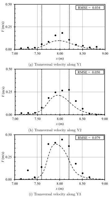
av-erage RMSE = 0.005. The simulated depth-avav-eraged streamwise velocity is in good
agreement with the experimental values (Figs. 4.2d, e and f) with little
overestima-tion at the end of secoverestima-tion Y1 (Fig. 4.2 d). This is due to the reflecoverestima-tion from the