https://doi.org/10.5194/nhess-19-1387-2019 © Author(s) 2019. This work is distributed under the Creative Commons Attribution 4.0 License.
Simultaneous state–parameter estimation of rainfall-induced
landslide displacement using data assimilation
Jing Wang1, Guigen Nie1,2, Shengjun Gao3, and Changhu Xue1 1GNSS Research Center, Wuhan University, Wuhan, 430079, China
2Collaborative Innovation Center for Geospatial Information Technology, Wuhan, 430079, China 3Chinese Antarctic Center of Surveying and Mapping, Wuhan, 430079, China
Correspondence:Guigen Nie ([email protected])
Received: 30 January 2019 – Discussion started: 7 February 2019
Revised: 30 May 2019 – Accepted: 3 June 2019 – Published: 11 July 2019
Abstract.Landslide displacement prediction has great prac-tical engineering significance to landslide stability evalua-tion and early warning. The evoluevalua-tion of landslide is a com-plex dynamic process, and applying a classical prediction method will result in significant error. The data assimila-tion method offers a new way to merge multisource data with the model. However, data assimilation is still deficient in the ability to meet the demand of dynamic landslide sys-tems. In this paper, simultaneous state and parameter esti-mation (SSPE) using particle-filter-based data assimilation is applied to predict displacement of the landslide. A land-slide SSPE assimilation strategy can make use of time-series displacements and hydrological information for the joint es-timation of landslide displacement and model parameters, which can improve the performance considerably. We select Xishan Village, Sichuan Province, China, as the experiment site to test the SSPE assimilation strategy. Based on the com-parison of actual monitoring data with prediction values, re-sults strongly suggest the effectiveness and feasibility of the SSPE assimilation strategy in short-term landslide displace-ment estimation.
1 Introduction
Landslide is a common geological hazard which greatly en-dangers the security of property and lives of the people (Huang et al., 2017; Froude and Petley, 2018; Zhang and Huang, 2018; Pham et al., 2018). The landslide in Sri Lanka in May 2017 resulted in more than 200 casualties and injured 698 289 people. (Kumarasiri, 2018). In China alone,
land-slide hazards account for about 72.6 % of the total geological disasters from 2005 to 2014 (Xue et al., 2016). Therefore, landslides are important to study, lending themselves for pre-vention studies like early warning systems and deformation predictions (Liu et al., 2014; Jiang et al., 2016; Michoud et al., 2016).
continu-ously distributed over time and space (Xue et al., 2018). Data assimilation has been widely tested and used in geoscience fields like hydrologic and atmospheric sciences (Reichle et al., 2002; Abbaszadeh et al., 2017; Wikle, 2002). And al-though very promising, there have been only a few prelimi-nary studies using data assimilation techniques that involve studying landslides.
Data assimilation can be divided into two types: the sequential-based method and the continuous-based method (Qin et al., 2009). The sequential-based method is an online approach that updates the prediction each time (Nakano et al., 2007), so it is more suitable for landslide systems than the continuous-based method. A particle filter (PF) is a typical sequential data assimilation algorithm which was initially put forward by Gordon (Gordon et al., 2002). Because the PF is nonlinear filtering based on Bayesian estimation, it can solve nonlinear and non-Gaussian problems (Moradkhani and Wei-hermüller, 2011). Landslides and parameters that describe landslides are typically nonlinear (Leeuwen, 2010), so we choose PF as the algorithm to integrate multisource data with the model.
The evolution of a landslide is a time-varying process, so the model parameters are required to be adjusted over time. However, primal sequential data assimilation only updates state vectors, and the model parameters are generally given by known information, which will result in discrepancies be-tween state and model parameters under a particular model relationship (Nearing et al., 2012). To meet the requirements of updating state values and model parameters simultane-ously, we apply the simultaneous state and parameter esti-mation (SSPE) here. The SSPE method can continuously re-new the output by sequentially merging re-new measurements. Moradkhani et al. (2005) optimized this process in the hydro-logical field. Vrugt et al. (2006) combined the simultaneous optimization with data assimilation. Joint estimation of the state parameter has proven to be a useful strategy to improve prediction performance (Qin et al., 2009; Lü et al., 2011).
In this paper, we applied the SSPE assimilation strategy to predict landslide displacement. In landslide SSPE assimila-tion, an external factor, hydrological data, has been integrated into the dynamic model of landslide deformation data, which can adjust model parameters and the state vector simultane-ously according to the hydrologic information. During the process, internal factors of a landslide are combined with ex-ternal observation factors, reducing the simulation error.
First, we will present the applied research method by de-scribing the time-series decomposition and how we estab-lished the model and landslide SSPE assimilation strategy applying the PF algorithm. The Xishan Village landslide is used here as the study area to examine the SSPE assimilation strategy. The prediction of deformation will be optimized by coupling GPS observation data with a hydrological factor. Finally, we will present and discuss the results.
2 Method
2.1 Time-series displacement decomposition
Landslide deformation is the interaction between internal ge-ological conditions and the external environment (Desai et al., 1995). Therefore the displacement can be divided into (a) a trend-term displacement generated by internal factors, (b) a periodic-term displacement caused by external fac-tors (such as rainfall and reservoir water level) and (c) a stochastic-term displacement (human impacted, snowpack, etc.) (Zhou et al., 2016). However, after noise filtering, the stochastic term is too small and can be neglected. So the time-series displacement decomposition is as follows:
S(i)=ϕ(i)+x(i), (1)
where S(i) is the cumulative displacement of landslides,
ϕ(i)denotes the trend term and x(i) denotes the periodic term.
The trend term of time series is extracted with the moving average method because it can remove the disturbance effec-tively and leave long-term signals for research (Seng, 2013).
ϕi=
Si−1+Si−2+ · · ·Si−n
n , (2)
whereϕiis the periodic term of stepi,Si−1is the cumulative displacement of stepi−1 andnis the moving average period. So the periodic-term displacement can be calculated by subtracting the trend term from the total displacement. 2.2 Landslide periodic displacement modeling
For rainfall-induced landslides, atmospheric rainfall is one of the most susceptible disaster-causing factors and directly af-fects the periodic displacement of a landslide (Lian et al., 2015; Ren et al., 2015). So the periodic term can be re-garded as a function of time and rainfall. The numerical func-tion method is adopted here to establish a periodic displace-ment model. The periodic displacedisplace-ment variation is minimal for short periods of time. Therefore, the model can be de-rived through expanding periodic displacement value using a Taylor-series expansion method:
x (ti+1, ri+1)=x (ti, ri)+
∂x ∂t
ti
(ti+1−ti)
+1 2
∂2x
∂t2
ti
(ti+1−ti)2+
∂x ∂r
ri
(ri+1−ri)
+1 2
∂2x
∂r2
ri
(ri+1−ri)2+gi,
derivative of displacement, ∂2x ∂t2 and
∂2x
∂r2 are the second-order
partial derivative, andgi is the remainder of Taylor’s expan-sion.
2.3 Landslide SSPE assimilation strategy using PF 2.3.1 State estimation
The general state-space model for a nonlinear dynamic sys-tem is defined to be
State model: xi+1=f (xi, ui)+vi+1, (4) Observation model: yi+1=g (xi+1)+wi+1, (5)
wherex is the state vector andy is the observation vector,
iis a time step,f andgare nonlinear functions forecasting the state and observation,urepresents the model parameters,
vis the model error andwis observation noise.
2.3.2 Landslide SSPE method
In sequential data assimilation, the SSPE algorithm can be applied through the state augmentation method (Chen et al., 2005). Considering the model in Eq. (4), the original state vectorxi is now augmented with the parametersu(t )to be
Xi=
xi
ui
. (6)
By incorporating the simultaneous state–parameter estima-tion method into the practical landslide state model Eq. (3), the extended state vector can be expressed as
Xi=
" x (ti, ri)
∂x ∂t ti
∂2x ∂t2 ti ∂x ∂r ri
∂2x ∂r2
ri #T
. (7)
And we set
∂x ∂t
ti+1
= ∂x ∂t ti +
∂2x
∂t2
ti
(ti+1−ti)+mi, (8)
∂2x
∂t2
ti+1
=
∂2x
∂t2
ti
+ni, (9)
∂x ∂r
ri+1
= ∂x ∂r ri +
∂2x
∂r2
ri
(ri+1−ri)+ui, (10)
∂2x
∂r2
ri+1
=
∂2x
∂r2
ri
+vi, (11)
wheremi,ni,uiandvi are noise.
So the next momentXi+1is
Xi+1=
x ti+1,ri+1
∂x ∂t
ti+1
∂2x ∂t2
ti+1
∂x ∂r
ri+1
∂2x
∂r2
ri+1
=
x (ti, ri)+
∂x
∂t
ti
(ti+1−ti)+ 1 2
∂2x
∂t2
ti
(ti+1−ti)2
+
∂x ∂r
ri
(ri+1−ri)+ 1 2
∂2x
∂r2
ri
(ri+1−ri)2+gi
∂x ∂t
ti +
∂2x
∂t2
ti
(ti+1−ti)+mi
∂2x ∂t2
ti +ni
∂x ∂r
ri +
∂2x
∂r2
ri
(ri+1−ri)+ui
∂2x
∂r2
ri +vi
=
1 ti+1−ti
1
2(ti+1−ti)
2 r
i+1−ri
1
2(ri+1−ri)
2
0 1 ti+1−ti 0 0
0 0 1 0 0
0 0 0 1 ri+1−ri
0 0 0 0 1
·
x (ti, ri)
∂x ∂t
ti ∂2x
∂t2 ti ∂x ∂r ri ∂2x
∂r2 ri + gi mi ni ui vi =
1 ti+1−ti 1
2(ti+1−ti) 2 r
i+1−ri 1
2(ri+1−ri) 2
0 1 ti+1−ti 0 0
0 0 1 0 0
0 0 0 1 ri+1−ri
0 0 0 0 1
·Xi+
In Eq. (12) we make
1 ti+1−ti 1
2(ti+1−ti) 2 r
i+1−ri 1
2(ri+1−ri) 2
0 1 ti+1−ti 0 0
0 0 1 0 0
0 0 0 1 ri+1−ri
0 0 0 0 1
=ωi+1,
gi mi ni ui vi
=εi+1,
so Eq. (12) can be expressed as
Xi+1=ωi+1·Xi+εi+1. (13)
The observation of landslide deformation can be expressed as
yi+1=xi+wi+1. (14)
Combining the two expressions, Eqs. (13) and (14), we can build the landslide SSPE state-space model to jointly esti-mate the landslide periodic displacement and the model pa-rameters.
2.3.3 PF algorithm
However, some parameters in the landslide state-space model, Eqs. (13) and (14), are difficult to obtain (e.g., ∂x∂tt
i,
∂2x ∂t2
ti
). By applying Monte Carlo simulations, the PF can be adjusted to solve this. Instead of calculating the partial derivative directly, PF generates a large number of samples (particles) to approximate the posterior probability of the states, thus obtaining an optimal result (Maskell and Gordon, 2002).
From the Bayesian theorem, the posterior probability of the states can be inferred through
1. forecast,
p (xi|y1:i−1)= Z
p (xi|xi−1) p (xi−1|y1:i−1)dxi−1, (15)
2. and update,
p (xi|y1:i)=
p yi|xip (xi|y1:i−1)
p yi|y1:i−1
, (16)
where i is time, xi is the state vector, yi is the ob-servation vector,y1:i = {y1, y2,· · ·,yi},p(xi−1|y1:i−1) is the posterior distribution function (PDF) for time stepi−1,p(xi|y1:i−1)is the prior distribution for time stepiandp(xi|xi−1)can be derived from the model.
In PF, the posterior probability of the states is approxi-mated by discrete random measures defined by particles and a set of weights associated with particles:
ˆ
p (xi|y1:i)≈ N
X
k=1
wkiδx0:i−x0k:i
, (17)
wherep(xˆ i|y1:i)is the approximate value ofp(xi|y1:i),x0k:i andwik are particles and associated weight,
N
P
i=1
wki =1 and
δdenotes the Dirac delta function.
Direct sampling of targetp(xi|y1:i)can be problematic, so sequential importance sampling (SIS) is considered here to overcome this. The SIS gathers particles from a known den-sity function and updates the importance weights by using an iterative method (Doucet et al., 2000). Meanwhile, the sam-pling importance resamsam-pling (SIR) is used to avoid particles deviates away from the true value (Gordon et al., 2002). The SIR algorithm gathers particles by their importance weight. So the estimates of the state vector can be described as
ˆ
xi= N
X
k=1
xkiwik. (18)
The procedure of the landslide SSPE assimilation strategy is shown in Fig. 1.
3 Study area and data 3.1 Study area
Our study area is located in Xishan Village, Li County, Sichuan Province, China (Fig. 2), in the upper part of the northern bank slope of the Zagunao River. The slope of this landslide is about 25–45◦. The length is about 4200 m, and the width is around 1700 m. The altitude of the leading edge is 1500 m, and the trailing edge is 3400 m. Thus the elevation is 1900 m. This landslide can be best described as a mas-sive accumulative landslide. It can be divided into three parts according to geomorphogenesis: (i) erosional with a dip di-rection of about 178◦, (ii) erosional and denudational with a dip direction of about 200◦, and (iii) glacial and periglacial with a dip direction of about 208◦. The distribution of the three parts is shown in Fig. 3. The Xishan landslide is a soft rock, layered structure slope. Exposed strata in the study area resemble mainly blue grey phyllite. The upper deposit is formed due to the collapse of slope and ice water accumu-lation and is mainly composed of silt and gravel soil.
Figure 1.The flow chart of the landslide SSPE assimilation strategy.
Figure 2.Location of the Xishan landslide in China(a); the Xishan landslides in the west of Wenchuan County associated with land-form. Map obtained from Google Earth(b).
deformation intensified after the Wenchuan earthquake (May 2008), which threatened the security of residents’ lives and properties. The estimated potential economic loss was about Yuan 50 million. For the purpose of reducing damage by pro-viding early warning, this study was used to forecast the de-formation of this landslide.
3.2 Data introduction
3.2.1 GPS-derived time-series displacement
Five continuous GPS observation stations have been set up for the Xishan Village landslide to obtain any deformation observations. The GPS receivers were connected to a net-work so the observations could be transferred in real time. At the same time, a GPS reference station was placed in a stable area and used for reference. Figure 3 shows the distri-bution of all stations. After the GPS baseline calculation, we calculated the deformation of every observation station from August 2015 to June 2017. Figure 4 shows the final results. Due to transmission problems, there are several gaps in the data. An interpolation method was applied to overcome these data gaps (Velicer and Colby, 2005; Lenda et al., 2016). 3.2.2 Rainfall data
There are two rain gauges on the landslide, which can trans-mit rainfall data in real time. Figure 3 shows the location of the rain gauges. Both are near GPS stations. The daily rainfall data are illustrated in Fig. 6. Since the rain gauges are located near the GPS station, the mean values of the two gauges are taken as the rainfall of the Xishan landslide.
4 Results and analysis
Figure 3.The distribution of the three parts (I–III), GPS stations and rain gauges at the Xishan landslide.
benchmarked with the SSPE method. The SSPE method only applied the SSPE strategy and updated the state value with Eq. (13), without using data assimilation to optimize model and state parameters. All the experimental data were ob-tained at the Xishan Village landslide between August 2015 and June 2017. We only present our findings for two stations, GPS03 and GPS04, because the deformation is more evident there. Due to the complex terrain and insufficient power sup-ply of Xishan Village, the monitoring GPS sequence con-tained significant noise or errors. In order to reduce the influ-ence of this, we need to modify the time step. After exper-iment and evaluation among different time steps, a 5 d time step gives the best correlation with rainfall data. Therefore the time step is set to 5 d. The predicted displacement can be separated by a trend term, a period term and a
cumula-Figure 4.The GPS-derived time-series displacement of the Xishan landslide.
tive term. Then the error analysis is taken to validate the effi-ciency of our method.
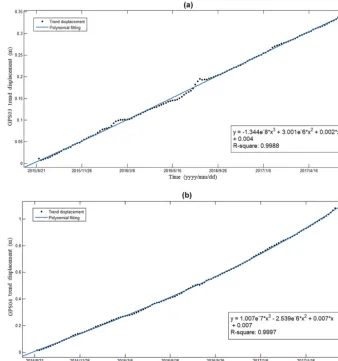
4.1 Prediction of trend-term displacement
The trend-term displacement is a time monotone function so that it can be fitted to a polynomial. The most optimal results of the trend-term prediction and the fitting formula are shown in Fig. 5.
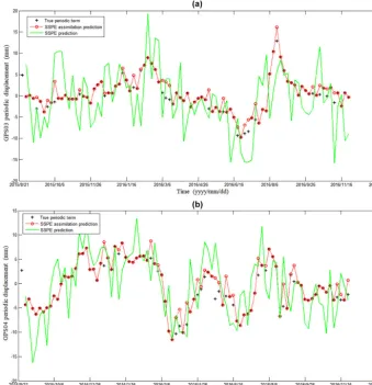
4.2 Prediction of period-term displacement
The periodic-term displacement can be calculated using the difference between the total displacement and the trend term. Figure 6 shows the periodic displacement in station GPS03 and GPS04 and the rainfall data. It can be seen clearly that the period term is a complex nonlinear sequence series. Be-sides, fluctuation of the period term of the two stations shows relatively the same changing tendency for both, which lags behind that of rainfall. However, there are small differences in fluctuation like time step 40 to 50 and 70 to 76. This could be attributed to the impact of geology. The GPS04 sta-tions monitor the first part of the landslide. There are a large number of people living here. The combined contribution of surface water, domestic water and ground water reduces the friction of the sliding belt, thus leading to drastic distortion. Station GPS03 monitors part III, the upper part of the land-slide (Fig. 3). This part with rare plant cover is susceptible to heavy rainfall season.
We applied the SSPE assimilation method to predict pe-riodic displacement. The prediction results are as shown in Fig. 7. It can be seen that the SSPE assimilation method gets closer to the measured value than the SSPE method without assimilation.
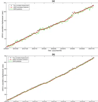
4.3 Prediction of cumulative displacement
Figure 5.The trend-term displacement prediction of(a)station GPS03 and(b)station GPS04.
Figure 6.The periodic-term displacement combined with rainfall data in GPS03 and GPS04.
Experimental results verify the feasibility of the SSPE assim-ilation method.
4.4 Relative error analysis
Figure 7.The periodic-term displacement prediction of(a)station GPS03 and(b)station GPS04.
Table 1.Comparison between the predicted values of cumulative displacement and measured displacement using different methods in station GPS03.
Time Measured SSPE SSPE assimilation
(mm) Prediction Difference Error Prediction Difference Error
(mm) (mm) rate (mm) (mm) rate
(%) (%)
11 Oct 2015 32.2674 40.2287 −7.9614 −24.67 29.1589 3.1085 9.63 16 Dec 2015 63.3499 68.1207 −4.7708 −7.53 61.8590 1.4909 2.35 6 Apr 2016 116.0395 105.4518 10.5878 9.12 115.0090 1.0305 0.89 11 Jun 2016 144.7729 133.5143 11.2586 7.78 145.9559 −1.1830 −0.82 6 Jul 2016 157.6520 146.3509 11.3011 7.16 156.2981 1.3539 0.86 11 Aug 2016 191.482 180.9944 10.4876 5.48 190.1751 1.3069 0.68 16 Oct 2016 215.3067 224.5674 −9.2607 −4.30 215.4657 −0.1590 −0.07 21 Nov 2016 233.1672 220.3506 12.8166 5.49 231.5734 1.5938 0.68
absolute error (MAE), mean squared error (MSE) and root mean square error (RMSE) – were used to evaluate the pre-diction effect. They can measure the deviation between the predicted value and the measured value and are calculated by
MAE= 1
N ·
N
X
i=1
xi− ˆxi
Figure 8.The cumulative displacement prediction of(a)station GPS03 and(b)station GPS04.
Table 2. Comparison between the predicted values of cumulative displacement and measured displacement using different methods in station GPS04.
Time Measured SSPE SSPE assimilation
(mm) Prediction Difference Error Prediction Difference Error
(mm) (mm) rate (mm) (mm) rate
(%) (%)
26 Dec 2015 189.1781 175.2549 13.9232 7.36 180.9129 8.2652 4.37 21 Feb 2016 261.1626 252.4146 8.7480 3.35 260.5177 0.6449 0.25 1 Apr 2016 304.7420 296.5933 8.1486 2.67 301.3644 3.3775 1.11 6 Jun 2016 402.9618 394.7279 8.2339 2.04 400.5510 2.4108 0.60 1 Aug 2016 492.6282 479.9417 12.6865 2.58 484.7087 7.9195 1.61 26 Sep 2016 572.1082 559.3349 12.7733 2.23 564.2868 7.8214 1.37 11 Nov 2016 646.0208 636.9418 9.0790 1.41 642.0225 3.9983 0.62
MSE= 1
N ·
N
X
i=1
xi− ˆxi 2
, (20)
RMSE=
v u u t
1
N ·
N
X
i=1
xi− ˆxi
2
, (21)
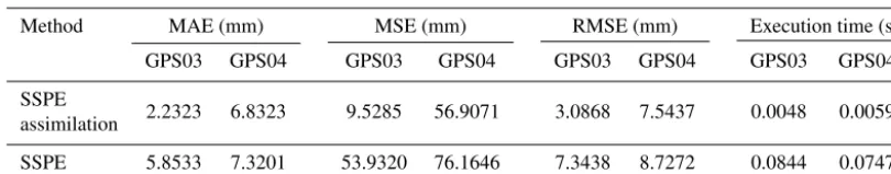
Table 3.Comparison of mean absolute error (MAE), mean squared error (MSE) and root mean square error (RMSE) performance and needed time using different methods in two stations.
Method MAE (mm) MSE (mm) RMSE (mm) Execution time (s)
GPS03 GPS04 GPS03 GPS04 GPS03 GPS04 GPS03 GPS04
SSPE
2.2323 6.8323 9.5285 56.9071 3.0868 7.5437 0.0048 0.0059 assimilation
SSPE 5.8533 7.3201 53.9320 76.1646 7.3438 8.7272 0.0844 0.0747
SSPE method in GPS03 station, respectively, and 6.66 %, 25.28 % and 13.56 % lower in GPS04 station, respectively. The result suggests that the SSPE assimilation method has achieved great performance in landslide displacement pre-diction. Besides, the total execution time of the two meth-ods is calculated. Building the SSPE model for landslide displacement prediction only takes 0.0048 and 0.0059 s for the two stations, while the SSPE assimilation strategy takes 0.0844 and 0.0747 s. It can therefore be considered as a near-real-time solution to make a displacement prediction simul-taneously.
5 Conclusion
This paper presents a practical strategy for accurately pre-dicting landslide displacement by coupling landslide defor-mation with external factors. For this, the PF data assimi-lation algorithm was integrated with the SSPE method. For the real data experiment, first the landslide deformation from GPS measurements was decomposed into a trend term and a period term. The period term was predicted with the hydro-logical factor in simultaneous estimation data assimilation, while the trend term was computed by polynomial fitting.
Our results show that the SSPE assimilation strategy has an excellent ability to predict landslide displacement and can provide assistance in early risk assessment and landslide forecasting.
Data availability. The data used in this paper are part of a national project. For this reason, the data are not available online but can be accessed by contacting the corresponding author.
Author contributions. JW proposed the idea, planned the experi-ment and completed this article. GN provided financial support for this research. SG assisted with the drawing of the pictures. CX helped submit the work.
Competing interests. The authors declare that they have no conflict of interest.
Special issue statement. This article is part of the special issue “Ad-vances in computational modeling of natural hazards and geohaz-ards”. It is a result of the Geoprocesses, geohazards – CSDMS 2018, Boulder, USA, 22–24 May 2018.
Acknowledgements. We thank the editor and the anonymous re-viewers. The authors acknowledge Google Earth for providing the map.
Financial support. This research has been supported by the Na-tional Program on Key Basic Research Project of China (grant no. 2013CB733205).
Review statement. This paper was edited by Albert J. Kettner and reviewed by two anonymous referees.
References
Abbaszadeh, P., Moradkhani, H., and Yan, H.: Enhancing Hy-drologic Data Assimilation by Evolutionary Particle Filter and Markov Chain Monte Carlo, Adv. Water Resour., 111, 192–204, https://doi.org/10.1016/j.advwatres.2017.11.011, 2017. Chaussard, E., Wdowinski, S., Cabral-Cano, E., and Amelung,
F.: Land subsidence in central Mexico detected by ALOS InSAR time-series, Remote Sens. Environ., 140, 94–106, https://doi.org/10.1016/j.rse.2013.08.038, 2014.
Chen, T., Morris, J., and Martin, E.: Particle filters for state and parameter estimation in batch processes, J. Process. Contr., 15, 665–673, https://doi.org/10.1016/j.jprocont.2005.01.001, 2005. Crosta, G. B., Frattini, P., and Agliardi, F.: Deep seated gravitational
slope deformations in the European Alps, Tectonophysics, 605, 13–33, https://doi.org/10.1016/j.tecto.2013.04.028, 2013. Desai, C. S., Samtani, N. C., and Vulliet, L.: Constitutive
Model-ing and Analysis of CreepModel-ing Slopes, J. Geotech. Eng., 122, 43– 56, https://doi.org/10.1061/(ASCE)0733-9410(1995)121:1(43), 1995.
Doucet, A., Godsill, S., and Andrieu, C.: On sequential monte carlo sampling methods for bayesian filtering, Statist. Comput., 10, 197–208, https://doi.org/10.1023/A:1008935410038, 2000. Froude, M. and Petley, D.: Global fatal landslide occurrence
from 2004 to 2016, Nat. Hazards Earth Syst. Sci., 18, 2161–2181, https://doi.org/10.5194/nhess-18-2161-2018, 2018.
Gordon, N. J., Salmond, D. J., and Smith, A. F. M.: Novel approach to nonlinear/non-Gaussian Bayesian state estima-tion, IEEE Proc. F-Radar Signal Process., 140, 107–113, https://doi.org/10.1049/ip-f-2.1993.0015, 2002.
Huang, F., Huang, J., Jiang, S., and Zhou, C.: Landslide dis-placement prediction based on multivariate chaotic model and extreme learning machine, Eng. Geol., 218, 173–186, https://doi.org/10.1016/j.enggeo.2017.01.016, 2017.
Jiang, Y. N., Liao, M. S., Zhou, Z. W., Shi, X. G., Zhang, L., and Balz, T.: Landslide Deformation Analysis by Coupling De-formation Time Series from SAR Data with Hydrological Fac-tors through Data Assimilation, Remote Sens., 8, 179–200, https://doi.org/10.3390/rs8030179, 2016.
Kumarasiri, W. K.: Damage and loss assessment of Landslide Dis-asters in Sri Lanka – A case study based on Landslide DisDis-asters in May 2017, in: Proceedings of the 8th Annual NBRO Sympo-sium, January 2018, Colombo, Sri Lanka, 2018.
Lee, E.-J., Liao, W.-Y., Lin, G.-W., Chen, P., Mu, D. W., and Lin, C.-W.: Towards Automated Real-Time Detection and Location of Large-Scale Landslides through Seismic Waveform Back Projec-tion, Geofluids, 1, 1–14, https://doi.org/10.1155/2019/1426019, 2019.
Leeuwen, P. J. V.: Nonlinear data assimilation in geosciences: an extremely efficient particle filter, Q. J. Roy. Meteorol. Soc., 136, 1991–1999, https://doi.org/10.1002/qj.699, 2010.
Lenda, G., Ligas, M., Lewi´nska, P., and Szafarczyk, A.: The use of surface interpolation methods for landslides monitoring, KSCE J. Civ. Eng., 20, 188–196, https://doi.org/10.1007/s12205-015-0038-4, 2016.
Li, H., Xu, Q., He, Y., and Deng, J.: Prediction of land-slide displacement with an ensemble-based extreme learn-ing machine and copula models, Landslides, 15, 2047–2059, https://doi.org/10.1007/s10346-018-1020-2, 2018.
Li, X. Z. and Kong, J. M.: Application of GA-SVM method with parameter optimization for landslide development prediction, Nat. Hazards Earth Syst. Sci., 14, 525–533, https://doi.org/10.5194/nhess-14-525-2014, 2014.
Lian, C., Zeng, Z., Yao, W., and Tang, H.: Multiple neural networks switched prediction for landslide displacement, Eng. Geol., 186, 91–99, https://doi.org/10.1016/j.enggeo.2014.11.014, 2015. Liu, Z., Shao, J., Xu, W., Chen, H., and Shi, C.: Comparison on
landslide nonlinear displacement analysis and prediction with computational intelligence approaches, Landslides, 11, 889–896, https://doi.org/10.1007/s10346-013-0443-z, 2014.
Lü, H., Yu, Z., Zhu, Y., Drake, S., Hao, Z., and Sudicky, E. A.: Dual state-parameter estimation of root zone soil mois-ture by optimal parameter estimation and extended Kalman filter data assimilation, Adv. Water Resour., 34, 395–406, https://doi.org/10.1016/j.advwatres.2010.12.005, 2011. Maskell, S. and Gordon, N.: A tutorial on particle filters for on-line
non-linear/non-gaussian Bayesian tracking, IEEE T. Signal Pro-cess., 50, 174–188, https://doi.org/10.1049/ic:20010246, 2002.
Michoud, C., Baumann, V., Lauknes, T. R., Penna, I., Derron, M.-H., and Jaboyedoff, M.: Large slope deformations detection and monitoring along shores of the Potrerillos dam reservoir, Ar-gentina, based on a small-baseline InSAR approach, Landslides, 13, 451–465, https://doi.org/10.1007/s10346-015-0583-4, 2016. Moradkhani, H. and Weihermüller, L.: Hydraulic parameter estimation by remotely-sensed top soil moisture observa-tions with the particle filter, J. Hydrol., 399, 410–421, https://doi.org/10.1016/j.jhydrol.2011.01.020, 2011.
Moradkhani, H., Sorooshian, S., Gupta, H. V., and Houser, P. R.: Dual state–parameter estimation of hydrological models us-ing ensemble Kalman filter, Adv. Water Resour., 28, 135–147, https://doi.org/10.1016/j.advwatres.2004.09.002, 2005. Nakano, S., Ueno, G., and Higuchi, T.: Merging particle filter for
se-quential data assimilation, Nonlin. Processes Geophys., 14, 395– 408, https://doi.org/10.5194/npg-14-395-2007, 2007.
Nearing, G. S., Crow, W. T., Thorp, K. R., Moran, M. S., Reichle, R. H., and Gupta, H. V.: Assimilating remote sensing observations of leaf area index and soil moisture for wheat yield estimates: An observing system simulation experiment, Water Resour. Res., 48, 213–223, https://doi.org/10.1029/2011WR011420, 2012. Pham, B. T., Tien Bui, D., and Prakash, I.: Bagging based
Sup-port Vector Machines for spatial prediction of landslides, En-viron. Earth Sci., 77, 146–162, https://doi.org/10.1007/s12665-018-7268-y, 2018.
Qin, J., Liang, S., Yang, K., Kaihotsu, I., Liu, R., and Koike, T.: Simultaneous estimation of both soil moisture and model pa-rameters using particle filtering method through the assimilation of microwave signal, J. Geophys. Res., 114, D15103–D15115, https://doi.org/10.1029/2008JD011358, 2009.
Reichle, R. H., Mclaughlin, D. B., and Entekhabi, D.: Hydro-logic Data Assimilation with the Ensemble Kalman Filter, Mon. Weather Rev., 130, 103–114, https://doi.org/10.1175/1520-0493(2002)130<0103:HDAWTE>2.0.CO;2, 2002.
Ren, F., Wu, X., Zhang, K., and Niu, R.: Application of wavelet analysis and a particle swarm-optimized support vector ma-chine to predict the displacement of the Shuping landslide in the Three Gorges, China, Environ. Earth Sci., 73, 4791–4804, https://doi.org/10.1007/s12665-014-3764-x, 2015.
Seng, H.: A new approach of moving average method in time series analysis, in: 2013 Conference on New Media Studies (CoNMedia), Tangerang, 1–4, https://doi.org/10.1109/CoNMedia.2013.6708545, 2013. Velicer, W. F. and Colby, S. M.: A Comparison of
Missing-Data Procedures for Arima Time-Series Analysis, Educ. Psycholog. Meas., 65, 596–615, https://doi.org/10.1177/0013164404272502, 2005.
Vrugt, J. A., Gupta, H. V., Nualláin, B. Ó., and Bouten, W.: Real-Time Data Assimilation for Operational Ensem-ble Streamflow Forecasting, J. Hydrometeorol., 7, 548–565, https://doi.org/10.1175/JHM504.1, 2006.
Wikle, C. K.: Atmospheric Modeling, Data Assimila-tion, and Predictability, Technometrics, 47, 521–521, https://doi.org/10.1198/tech.2005.s326, 2002.
Xue, K., Yanxiang, H. U., Zou, Y., Tiwari, B., Wei, Y., and Gu, L.: Temporal-spatial distribution discipline of geological dis-aster in China in recent ten years, Chinese J. Geol. Hazard Control, 27, 90–97, https://doi.org/10.16031/j.cnki.issn.1003-8035.2016.03.14, 2016.
Yin, Y., Wang, H., Gao, Y., and Li, X.: Real-time monitoring and early warning of landslides at relocated Wushan Town, the Three Gorges Reservoir, China, Landslides, 7, 339–349, https://doi.org/10.1007/s10346-010-0220-1, 2010.
Zhang, F. and Huang, X.: Trend and spatiotemporal distribution of fatal landslides triggered by non-seismic effects in China, Landslides, 15, 1663–1674, https://doi.org/10.1007/s10346-018-1007-z, 2018.