Parametric Estimation in a Recurrent Competing Risks Model

Vol. 12, No. 1, pp 153-181

Parametric Estimation in a Recurrent

Competing Risks Model

Laura L. Taylor1_{, Edsel A. Pe˜na}2

1_{Department of Mathematics and Statistics, Elon University, Elon.}

2_{Department of Statistics, University of South Carolina, Columbia, NC, SC.}

Abstract. A resource-efficient approach to making inferences about the distributional properties of the failure times in a competing risks setting is presented. Efficiency is gained by observing recurrences of the compet-ing risks over a random monitorcompet-ing period. The resultcompet-ing model is called the recurrent competing risks model (RCRM) and is coupled with two repair strategies whenever the system fails. Maximum likelihood estima-tors of the parameters of the marginal distribution functions associated with each of the competing risks and also of the system lifetime dis-tribution function are presented. Estimators are derived under perfect and partial repair strategies. Consistency and asymptotic properties of the estimators are obtained. The estimation methods are applied to a data set of failures for cars under warranty. Simulation studies are used to ascertain the small sample properties and the efficiency gains of the resulting estimators.

Keywords. Competing risks, martingales, perfect and partial repairs, recurrent events, repairable systems, survival analysis.

MSC: Primary: 62N05; Secondary: 62F12.

1

Introduction

Consider a series or a competing risks system with Qcomponents. De-note by T1, T2, . . . , TQ the (possibly latent) times-to-failure of the Q

Laura L. Taylor( )([email protected]), Edsel A. Pe˜na([email protected]) Received: October 31, 2011; Accepted: July 17, 2012

components. To avoid identifiability issues (cf., Tsiatis [17] and Heck-man and Honor´e [7]), these variables are assumed to be independent. Additionally, letFq(·) be the distribution ofTq, which in this paper will

be assumed continuous. The system life is denoted byS, the minimum of theTq’s. In terms ofF1, F2, . . . , FQ, the system life distribution, FS,

is given by

FS(s) =P(S≤s) = 1− Q

∏

q=1

[1−Fq(s)]. (1)

Let Λq be the cumulative hazard function associated with Fq so that

Λq(t) =−log(1−Fq(t)), q= 1,2, . . . , Q,

and letλq be its associated hazard rate function whereλq=fq/(1−Fq)

with fq the density function of Fq. These functions are related to the

qth cumulative incidence function or sub-distribution function (cf., [10]), defined via ˘Fq(t) =P{S ≤t, S =Tq}, according to the relationship

˘

Fq(t) =

∫ t

0

¯

FS(w)Λq(dw).

In the competing risks literature, there is also the notion of a cause-specific hazard rate function associated with the qth risk defined via

˘

λq(t) = lim

∆t↓0

1

∆tP{S ∈[t, t+dt), S =Tq|S≥t}, q= 1,2, . . . , Q.

By virtue of the assumed independence of theTq’s, note that we have the

identities λq(·) = ˘λq(·) for q = 1,2, . . . , Q. Since the qth cause-specific

cumulative hazard function is defined via ˘Λq(t) =

∫t

0λ˘q(w)dw, then this

equals Λq(t) under the independence assumption among theTq’s. Note,

however, that it is notthe case that ˘Λq=−log(1−F˘q) whenQ >1.

For purposes of making inference about FS, and of the Fq’s or the

˘

Fq’s, n independent systems or units will be monitored. The ith

sys-tem will be under observation during the random period [0, τi]. The

monitoring times, τ1, τ2, . . . , τn, are assumed to be independent with

common distribution function G, which is non-informative about the

Fq’s. The τi’s are also assumed to be independent of the inter-failure

times. In the usual competing risks model, theith system is monitored either until its system failure Si or until τi. It is assumed that when

the system fails, the component that caused the failure could be deter-mined. In this basic competing risks model, the random observables

are {(Zi, δi), i = 1,2, . . . , n}, where Zi = min(Si, τi); δi = 0 whenever

Zi =τi, so the system lifeSi is right-censored byτi; andδi=qwhenever

Zi =TiqwithTiqthe latent time-to-failure due to causeq, so theith

sys-tem failed due to the failure of component q which happened before τi.

Theδi’s are the indicator variables of the component that caused system

failure. Given these random observables, inference about the individual

Fq’s are made which may lead to a better inference about the system life,

FS, by exploiting equation (1). If interest is on the cause-specific

sub-distribution functions ˘Fq’s, then estimators of these functions could be

obtained from the estimators of ¯FSand the Λq’s. This basic model is the

so-called single-event competing risks model, which has been considered in Crowder [5] and will be hereon abbreviated SCRM.

Such studies may not, however, be resource-efficient. It is possi-ble that a system will fail early during the monitoring period [0, τi]

and, in the above scheme, this system will not anymore be monitored. The unfailed components in this system are in essence wasted. A more resource-efficient scheme may potentially be achieved by instituting a repair strategy after each system failure, similar in spirit to the idea of testing “with replacement” in [11]. Instead of discarding the system, a repair can be performed that may require either the entire system be replaced or the failed component that caused system failure be replaced by a new component. These types of repairs are, respectively, referred to as perfect repairs and partial repairs (cf., Bedford and Lindqvist [2]). Whichever repair strategy is adopted for the ith system is then con-tinuously implemented for this system during the random monitoring period [0, τi]. It will be assumed for simplicity, but clearly

unrealisti-cally, that the repair process of the system or the failed component can be performed instantaneously. The time of the jth failure for the ith system will be denoted bySij, while the associated event indicator will

be denoted by δij. For the ith system, the random number of system

failures over [0, τi] caused by theqth risk or component will be denoted

by Kiq. Observe that in this recurrent competing risks framework, in

contrast to the basic competing risks model, the period [Si1, τi] will still

be utilized to continue the monitoring of system i, which may provide more information leading to improved inferences regarding theFq’s and

consequently the system life distributionFS.

We shall refer to this model as the recurrent competing risks model (RCRM). Note that a recurrent competing risks model has been men-tioned in [4] in the context of analyzing data pertaining to recurrent failures of internal shunts described in [12, 18]. This RCRM offers a

more efficient use of the monitoring period to maximize the informa-tion obtained about the system life and the latent failure times. The primary goal of this paper is to obtain estimators of the marginal dis-tribution functions of each of the competing risks failure times and of the system life distribution under a perfect repair RCRM and a par-tial repair RCRM. We restrict the coverage of this paper to parametric models without covariates and defer the development of nonparametric methods and models with covariates for future work.

The context of application of the methods presented in this paper are expected to be useful in reliability and engineering settings where a parametric assumption may be appropriate. However, further exten-sions of the model should be made for many realistic applications to biomedical data that incorporate dependencies across risks. In partic-ular, a relaxation of the independence assumption of the Tq’s may be

needed to account for the deterioration of a system resulting from com-bined effects of other risks. Heckman and Honor´e [7] present conditions and models that induce identifiability. Their results were extended re-cently by Abbring and van den Berg [1]. Other avenues for modeling competing risks have incorporated copulas. These methods have been explored by Zheng and Klein [19] and subsequently by Lo and Wilke [13].

We outline the contents of this paper. Section 2 presents a math-ematical framework for the RCRM. Section 3 provides the maximum likelihood estimators of the model parameters. Gains in efficiency of the estimation procedure based on the RCRM relative to the non-recurrent SCRM are presented in Section 4. In Section 5, the estimation procedure is applied to a data set on failures of cars under warranty. To get an immediate idea of the type of data of interest, see Figure 5 on page 172, which is a graphical depiction of the car warranty data analyzed in Sec-tion 5. Small sample properties of the estimators are obtained through a simulation study in Section 6. Concluding remarks are provided in Section 7.

2

Recurrent Competing Risks Model

As mentioned in the preceding section, we will consider the situation where n systems or units are under consideration. For the ith system, the observable random vector will be

Di≡(Ki, τi, Si1, Si2, . . . , Si,Ki, τi−Si,Ki, δi1, δi2, . . . , δi,Ki),

where Ki = max{k: Sik ≤τi} is the total number of events (failures)

over [0, τi]. Observe that Ki is random and will be informative about

the Fq’s and FS. The random number of failures attributed to risk

q is Kiq =

∑Ki

j=1I{δij = q}. From Di, the inter-event times can be

recovered via Tij = Sij −Si,j−1 with Si0 ≡ 0. For the partial repair

model, successive calendar times are additionally denoted for risk q by

Sijq, j = 1,2, . . . , Kiq, and the inter-event times for risk q are given by

Tijq=Sijq−Si,j−1,q, j= 1,2, . . . , Kiq, withSi0q ≡0. [For our notation,

we shall on occasion write Ti,j,q for Tijq and Si,j,q for Sijq for clarity.]

Under the perfect repair model, thejth inter-event time associated with risk q, denoted by Tijq, will only be observed if the jth system failure

is due to risk q. In such a case, the inter-event times Tijv, v ̸= q, will

all be right-censored by Tijq. In addition, for the perfect repair model,

the inter-event times Ti,Ki+1,q, q= 1,2, . . . , Q, will all be right-censored

by τi−Si,Ki; while for the partial repair modelτi−Si,Kiq,q will be the

right-censoring variable forTi,Kiq+1,q for each q.

Assume theTijq’s are independent, and for a fixedq, are iid from an

unknown marginal distribution functionFqwhich belongs to a

paramet-ric family of distributionsCq ={Fq(·;θq) :θq∈Θq}whereΘqis an open

subset ofℜpq _whereP

qdenotes the number of parameters associate with

Fq. The marginal hazard rate function is denoted by λq(·;θq), whereθq

is a vector of distinct parameters associated with λq. As noted earlier,

by virtue of the independence of the latent variables, this marginal haz-ard rate function is also the cause-specific hazhaz-ard rate function. The parameter vector of interest is the p_•×1 vector θ = (θT₁,θT₂, . . . ,θT_Q)T_,

wherep_•=∑Q_q=1pq. Observe that

λq(t;θq) =

fq(t;θq)

Sq(t;θq)

, q= 1,2, . . . , Q,

wherefq(t;θq) is the marginal density associated with the marginal

dis-tribution function, Fq(t;θq) =P(Tijq ≤t) and Sq(t;θq) = 1−Fq(t;θq).

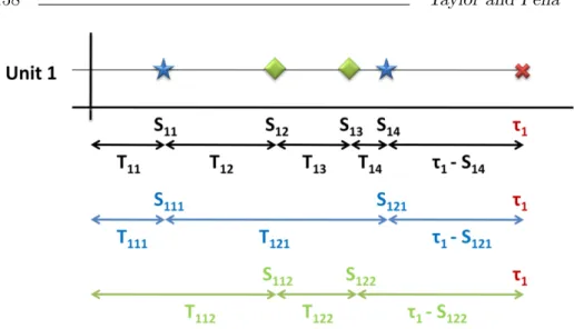
Therefore, it will suffice to estimate the parameters associated with the marginal hazard function in order to estimate the marginal distribu-tion funcdistribu-tion. Figure 1 illustrates the observed data for two recurrent competing risks under a partial repair model. The calendar times of fail-ures for the two competing causes are denoted by blue stars and green diamonds with the censoring time denoted by a red X. The observed system calendar times (Sij) and system inter-event times (Tij) are shown

in black. The observed calendar times (Sijq) and inter-event times (Tijq)

for each of the two causes are depicted in their associated colors as well.

Figure 1: Observable quantities for data generated from two recurrent competing risks under a partial repair strategy for one system.

3

Maximum Likelihood Estimation

3.1 Likelihood and Estimators

The main focus of this paper is the estimation of the parameter vector θ associated with the Q marginal distribution functions. To achieve more generality, we employ counting processes and martingales in the following. We shall define a generic counting process N_iq† = {N_iq†(s) :

s≥0}, which counts the number of failures due to causeq for system i

during calendar time period [0, s], which will vary depending on whether we have perfect or partial repair. For the perfect repair model (E) and for the partial repair model (A) this counting process becomes, respectively,

N_iqE(s) =

Ki ∑

j=1

I{Sij ≤s∧τi, δij =q} and NiqA(s) = Kiq ∑

j=1

I{Sijq≤s∧τi},

for i = 1,2, . . . , n and q = 1,2, . . . , Q. The at-risk process, Y_i†(s) =

I{τi ≥ s}, indicates whether unit i is still under observation at time

s. Additionally, define a generic backward recurrence process E_iq† =

{E_iq†(s) :s≥0}, which for the perfect repair model (E) and the partial repair model (A) becomes, respectively,

E_iqE(s) =s−S_i,NE

i (s−) and E

A

iq(s) =s−Si,N_iqA(s−),q,

where N_iE(s) = ∑Q_q=1N_iqE(s). Under the perfect repair model, E_iqE(s) is the time elapsed since the most recent failure due to any risk; while under the partial repair model,E_iqA(s) is the time elapsed since the most recent failure due to risk q only.

The filtration that is augmented to the basic probability space (Ω,F, P) on which all random entities are defined isF={Fs : s≥0}, where

Fs is the σ-field containing all information up to times, defined via

Fs=F0∨

{ _n ∨

i=1 σ

{(

N_iq†(v), Y_i†(v+)

)

:q = 1,2, . . . , Q; 0≤v≤s }}

,

where F0 is the σ-field containing all the information available at time

0.

Proposition 3.1. The intensity process of N_iq† with respect to F is Y_i†(s)λq(Eiq†(s);θq), that is, with dNiq†(s) = Niq†((s+ds)−)−Niq†(s−),

lim0<ds→0(ds)−1P {

dN_iq†(s) = 1|Fs−

}

=Y_i†(s)λq(E_iq†(s);θq).

Proof. For infinitesimal ds > 0, there will either be no failures or exactly one failure in [s, s+ds). Now, P(dN_iq†(s) = 1|Fs−) is the

con-ditional probability, given Fs−, of exactly one failure for the ith system

that is due to cause q in the interval of time [s, s+ds). We have for such a dsthat

P(dN_iq†(s) = 1|Fs−) =P{dNiq†(s) = 1;∩q′̸=q[dNiq†′(s) = 0]|Fs−}

= (Y_i†(s)λq(Eiq†(s);θq)ds+o(ds))

×

s_∏+ds v=s

  1−

∑

q′̸=q

λq′(Eiq†′(v);θq′)dv

  

= (Y_i†(s)λq(Eiq†(s);θq)ds+o(ds))

×exp

  −

∫ s+ds s

∑

q′̸=q

λq′(Eiq†′(v);θq′)dv

  

= (Y_i†(s)λq(Eiq†(s);θq)ds+o(ds))

×exp

  −

∑

q′̸=q

[Λq′(Eiq†′((s+ds)−);θq′)−Λq′(Eiq†′(s−);θq′)]

  ,

where ∏ denotes product integral. Dividing by dsand then taking the limit asds→0, the result follows since Λq′(E_iq†′(s);θq′) is left-continuous

ins.

The intensity process ofN_iq†(·) with respect toFisY_i†(·)λq(Eiq†(·);θq)

so that the process A†_iq ={A†_iq(s;θq) : s≥0}, defined by

A†_iq(s;θq) =

∫ s

0

Y_i†(v)λq(Eiq†(v);θq)dv,

is therefore the compensator ofN_iq†(s). By the Doob-Meyer decomposi-tion theorem,

{M_iq†(s;θq) =Niq†(s)−A†iq(s;θq) : s≥0}

is a zero-mean square-integrableF-martingale for eachiandq. The vec-torM†_i(v;θ) = (M_i†₁(v;θ1), . . . , M_iQ† (v,θQ))Tis aQ×1 vector of

square-integrable zero-mean martingale processes. Its predictable quadratic variation process is a diagonal matrix process with diagonal elements

⟨M_iq†⟩(s;θq) =A†iq(s;θq), q= 1,2, . . . , Q.

By results of Jacod [9], the full likelihood process at time sis given by

L(θ, s) =

s ∏ v=0 n ∏ i=1 Q ∏ q=1 {

[Y_i†(v)λq(E_iq†(v);θq)]dN

†

iq(v)

×[1−Y_i†(v)λq(E_iq†(v);θq)

]1−dN_iq†(v)}

= n ∏ i=1 Q ∏ q=1 {( _s ∏ v=0

[Y_i†(v)λq(Eiq†(v);θq)]dN

†

iq(v) ) ×exp { − ∫ s 0

Y_i†(v)λq(E†iq(v);θq)dv

}} .

Consequently, the log-likelihood process is{ℓ(θ, s) : s≥0} with

ℓ(θ, s) =

n ∑ i=1    ∫ s 0 Q ∑ q=1

log[Y_i†(v)λq(E_iq†(v);θq)]dN_iq†(v)

− ∫ s

0

Y_i†(v)

Q

∑

q=1

λq(E_iq†(v);θq)dv

  .

For purposes of obtaining the maximum likelihood estimators and their properties, we seek the p_•×1 score vector process U ={U(θ, s) :

s ≥ 0} and the p_• ×p_• observed information matrix process I(θ) =

{I(θ, s) : s≥0}. For this purpose, for a vector a, define the gradient operator∇a≡ _∂∂_a and, forq = 1,2, . . . , Q, let

ρ_q(s;θq) =∇θqlogλq(s;θq) and Vq(s;θq) =∇θT

q∇θqlogλq(s;θq).

Thus,ρ_q(s;θq) is apq×1 vector of functions, whileVq(s;θq) is apq×pq

matrix of functions.

Since the vector of score process is obtained viaU(θ, s) =∇θℓ(θ, s),

it is straightforward to obtain that the vector of score processes is U(θ, s) = (UT

1(θ1, s),UT2(θ2, s), . . . ,UTQ(θQ, s))T, whereUq(θq, s) is the

pq×1 vector given by

Uq(θq, s) = n

∑

i=1 ∫ s

0

ρ_q(E_iq†(v);θq)dMiq†(v;θq).

On the other hand, the observed Fisher information matrix process is defined via I(θ, s) = −∇_θTU(θ, s). It is straightforward to verify that

I(θ, s) is a block-diagonal matrix with the (q, q)th block matrix being thepq×pq matrix

Iqq(θq, s) = −∇θT

qUq(θq, s)

=

n

∑

i=1 ∫ s

0

Y_i†(v)ρ_q(E_iq†(v);θq)⊗2λq(Eiq†(v);θq)dv

−

n

∑

i=1 ∫ s

0

Vq(E_iq†(v);θq)dM_iq†(v;θq),

where for a vectora, we havea⊗2 =aaT_{. The ML estimator ofθ}

qbased

on the realization of the processes up to calendar times∗, denoted ˆθq(s∗),

is obtained as a solution of the equation

Uq(θq, s∗) =0. (2)

Numerical methods, such as the Newton-Raphson algorithm, will typi-cally be needed to obtain the estimate ˆθq(s∗) of θq based on equation

(2). The Newton-Raphson iteration is based on the updating ˆ

θnew_q ←θˆold_q +Iqq(ˆθ old

q , s∗)−1Uq(ˆθ old q , s∗).

3.2 Asymptotics

Asymptotic properties of ˆθ= (ˆθT₁,θˆT₂, . . . ,θˆT_Q)T_{, such as consistency and}

asymptotic normality, as n → ∞, follow from Borgan’s [3] results re-garding ML estimators from parametric counting process models. De-fine Iqq(θq, s) to be the in-probability limit of _n1Iqq(θq, s), and also let

I(θ, s) be the p_• ×p_• block-diagonal matrix with block-diagonal ele-ments Iqq(θq, s), q = 1,2, . . . , Q. Recalling the standard ‘asymptotic

normality’ notation (cf., [15]) that Tn∼AN(µn,Σn) means that

Σ−_n1/2(Tn−µn)−→d N(0,I),

we have that under certain regularity conditions, ˆ

θ(s∗)∼AN (

θ,1 nI(θ, s

∗₎−1 )

.

Because of the block-diagonal structure of I(θ, s∗), we can conclude that the ˆθq are asymptotically independent and also that for each q =

1,2, . . . , Q, we have ˆ

θq(s∗)∼AN

(

θq,

1

nIqq(θq, s

∗₎−1 )

.

A consistent estimator ofIqq(θq, s∗) obtained from the predictable

quad-ratic variation process of the score process is given by 1

n⟨Uq⟩(ˆθq, s

∗_{) =} 1

n

n

∑

i=1 ∫ s∗

0

ρ_q(E_iq†(v); ˆθq)⊗2Yi†(v)λq(Eiq†(v); ˆθq)dv. (3)

The estimate could be computed on a case-by-case basis depending on the form of the hazard rate functionλq.

For the purpose of getting exact efficiency expressions for some mod-els, we now seek an expression of Iqq(θq, s∗) for q = 1,2, . . . , Q. To

achieve a unified notation for the perfect and partial repair schemes, for

i= 1,2, . . . , n and q= 1,2, . . . , Q, let

S_i∗_0q = 0 and S_ijq∗ = inf{s > S_i,j∗ _−1,q : E_iq†(s) = 0};

K_iq∗(s∗) = max{j: S_ijq∗ ≤(s∗∧τi)};

T_ijq∗ =S_ijq∗ −S_i,j∗ _−1,q, j = 1,2, . . . , K_iq∗(s∗).

A generalized at-risk process could now be defined via

Y_iq∗(s∗, w) =

K_iq∗(s∗−) ∑

j=1

I{T_ijq∗ ≥w}+I{(s∗∧τi)−Si,K∗ _iq∗(s∗),q ≥w}.

Let us denote the expectation of this generalized at-risk process by

y_q∗(s∗, w;θ, G)≡y_q∗(s∗, w) =E{Y_iq∗(s∗, w)},

where G is the distribution of the censoring variable τ. Fortunately, not much work is needed since this expectation can be obtained from Proposition 1 of Pe˜na, Strawderman, and Hollander [14]. It follows that

1

n

n

∑

i=1

Y_iq∗(·, w)−→up y_q∗(·, w),

where ‘−→up ’ means uniform convergence in-probability on [0, s∗]. Analo-gously to the derivations in [14] using a change-of-variable in the integral, it follows that

Iqq(θq, s∗) =

∫ _∞ 0

y_q∗(s∗, w;θ, G)ρ_q(w;θq)⊗2λq(w;θq)dw.

Specializing to the perfect repair scheme, we have in this case that

T_ijq∗ = minq′=1,2,...,QTijq′, so the distribution function is identical to the

system life, which is

FS(t;θ) = 1− Q

∏

q=1

[1−Fq(t;θq)].

Thus, from [14], with Gs(t) =G(t)I{t < s}+I{t≥s}, it follows that

for this perfect repair scheme, y∗_q(s∗, t;θ, G) is equal to

y_qE(s∗, t;θ, G) = ¯FS(t;θ) ¯Gs∗(t) + ¯FS(t;θ)

∫ _∞

t

ϑS(w−t;θ)dGs∗(w),

whereϑS(·;θ) is the renewal function of FS(·;θ).

On the other hand, for the partial repair scheme, T_ijq∗ =Tijq whose

common distribution isFq(·;θq). Thus, again from [14], we obtain that

for this partial repair scheme, y∗_q(s∗, t;θ, G) is equal to

y_qA(s∗, t;θq, G) = ¯Fq(t;θq) ¯Gs∗(t) + ¯Fq(t;θq)

∫ _∞

t

ϑq(w−t;θq)dGs∗(w),

whereϑq(·;θq) is the renewal function ofFq(·;θq).

The estimation of the parameter vector of each of the component life distributions is perhaps more of secondary importance than the estima-tion of the system life distribuestima-tionFS. Upon obtaining the estimators of

theθq’s, we could now obtain an estimator ofFS by plugging-in ˆθq(s∗)

for θq in the expression for FS(t;θ) from equation (1) to obtain the

estimator ˆ

FS(s∗;t) =FS(t; ˆθ(s∗)) = 1− Q

∏

q=1

[1−Fq(t; ˆθq(s∗))].

By using the delta-method and noting that ˆθ(s∗) is asymptotically multi-variate normal with meanθand asymptotic covariance matrix 1_nI(θ, s∗)−1, it follows that for eacht≤s∗,

ˆ ¯

FS(s∗;t)∼AN

(

¯

FS(t;θ),

1

nσ 2

S(s∗;t;θ)

) ,

where

σ_S2(s∗;t;θ) = ¯FS(t;θ)2 Q

∑

q=1

•

Λq(t;θq)TIqq(θq, s∗)−1

•

Λq(t;θq)

withΛ•q (t;θq) =∇θqΛq(t;θq). We remark with regards to the notation

that when we lets∗→ ∞, we simply drop the arguments∗ in the above expressions. For example, ˆFS(s∗ =∞;t) will simply be written as ˆFS(t).

Since we would like to compare the gain in efficiency obtained by utilizing this RCRM relative to the SCRM, we recall that the associated ML estimator ofθfor the SCRM, denoted by ˜θ, is asymptotically multi-variate normal with meanθand asymptotic covariance matrix _n1I˜(θ)−1, where ˜I(θ) is the p_•×p_• block-diagonal matrix with (q, q)th block ma-trix given by thepq×pq matrix

˜

Iqq(θq) =

∫ _∞ 0

¯

FS(w;θq) ¯G(w)ρq(w;θq)⊗2λq(w;θq)dw.

Thus, if one only had data from the SCRM, an estimator ofFS(t;θ) will

be

˜

FS(t) =FS(t; ˜θ) = 1− Q

∏

q=1

[1−Fq(t; ˜θq)].

Using again the delta-method, it follows that for eacht, ˜

¯

FS(t)∼AN

(_¯

FS(t;θ),_n1σ˜2S(t;θ)

)

; ˜

σ2_S(t;θ) = ¯FS(t;θ)2

∑Q q=1

•

Λq(t;θq)TI˜qq(θq)−1

•

Λq(t;θq).

A measure of asymptotic relative efficiency (ARE) of the RCRM-based estimator ˆF¯S(t) relative to the SCRM-based estimator ˜F¯S(t) is given by

ARE( ˆF¯S(t) : ˜F¯S(t)) =

˜

σ2_S(t;θ)

σ2_S(t;θ) =

∑Q q=1

•

Λq (t;θq)TI˜qq(θq)−1

•

Λq (t;θq)

∑Q q=1

•

Λq (t;θq)TIqq(θq)−1

•

Λq (t;θq)

.

(4)

Theorem 3.1. The RCRM-based estimatorFˆ¯S(t), with either a perfect

repair or a partial repair strategy, dominates the SCRM-based estimator

˜ ¯

FS(t) in terms of asymptotic relative efficiency, that is, ARE( ˆF¯S(t) :

˜ ¯

FS(t))>1.0.

Proof. For the perfect repair strategy, this result is immediate from the fact that for eachq ∈ {1,2, . . . , Q}, we obtain from their respective expressions that IE_qq(θ) > I˜qq(θ). On the other hand, for the partial

repair strategy, by first noting that for each q′ = 1,2, . . . , Q, we have ¯

FS(t) =

∏Q

q=1F¯q(t) ≤ F¯q′(t), it follows that IAqq(θ) > I˜qq(θ), from

which the assertion of the theorem for the partial repair strategy follows.

4

Efficiency Comparisons

In this section we examine in concrete settings the magnitude of the gain in asymptotic efficiency when utilizing the RCRM versus the SCRM in estimating the system lifetime distribution FS. From Theorem 3.1 we

already know that the RCRM-based estimator will always be more ef-ficient than the SCRM-based estimator, so getting an idea of the mag-nitude of this efficiency improvement will provide us more information regarding the merits of adopting the RCRM design in real studies. We will consider two concrete situations: (i) when the component failure distributions are exponential and (ii) when the component failure dis-tributions are Weibull.

4.1 Exponential Component Lifetimes

Let us now assume that the component lifetime distributions are expo-nential, so thatFq(t;θq) = 1−exp(−θqt) fort≥0. We also assume that

G is exponential so that G(t;γ) = 1−exp(−γt) for t ≥0. Solving for

θq in the ML estimating equation in (2) yields the estimator

ˆ

θq(s∗) =

∑n

i=1Niq†(s∗)

∑n i=1

∫s∗

0 Yi†(v)dv

,

which is the occurrence-exposure rate under riskq. With θ_• =∑Q_q=1θq,

from [14] (see also [8]) we are able to obtain that

yE_q(w) = exp{−(θ_•+γ)w} (

1 +θ•

γ )

;

y_qA(w) = exp{−(θq+γ)w}

(

1 +θq

γ )

.

Straightforward calculations then yield that

I_qqE(θq) =

∫ _∞ 0

(

1 +θ•

γ )

e−(θ•+γ)w 1 θ2

q

θqdw=

1

θqγ

.

Similarly, we find that

I_qqA(θq) =

∫ _∞ 0

(

1 +θq

γ )

e−(θq+γ)w 1 θ2

q

θqdw =

1

θqγ

.

It is not surprising that these information values under the perfect and partial repair schemes are identical owing to the memoryless prop-erty of the exponential distribution. It follows therefore that under the assumption of exponential component lifetime distributions and an exponentially-distributed monitoring period, the RCRM-based estima-tors of ¯FS(t;θ) under either perfect or partial repair strategies satisfy

ˆ ¯

FS(t)∼AN

(

¯

FS(t;θ),

1

nt 2_θ

•γexp{−2tθ•}

) .

On the other hand, under the same distributional assumptions, the SCRM-based estimator of ¯FS(t;θ) satisfies

˜ ¯

FS(t)∼AN

(

¯

FS(t;θ),

1

nt 2_θ

•(θ_•+γ) exp{−2tθ_•} )

.

As a consequence, the asymptotic efficiency of ˆF¯S(t) relative to ˜F¯S(t)

under the exponential distribution assumptions is

ARE( ˆF¯S(t) : ˜F¯S(t)) = 1 +

θ_• γ = 1 +

E(τ)

E(S).

That is, the gain in efficiency using the RCRM over the SCRM, which is always positive, is solely determined by the ratio of the mean length of the monitoring period and the mean lifetime of the competing risk system.

4.2 Weibull Component Lifetimes

We were able to obtain an exact expression of the asymptotic relative efficiency of ˆF¯S(t) relative to ˜F¯S(t) under the exponential case because

of the fact that the renewal function of the exponential distribution is in closed-form, which for an exponential distribution with rate θ is given by ϑ(t) = θt. For many other distributions, such as the Weibull, no closed-form expressions of their renewal function are available, hence we are usually unable to obtain closed-form analytical expressions of asymptotic relative efficiencies. Thus, we resort to simulation studies to get an idea of the relative efficiencies under these non-exponentially distributed models.

Note also from equation (4) that the asymptotic relative efficiency of ˆF¯S(t) relative to ˜F¯S(t) will, in general, depend on the time t. To

examine the efficiency of the RCRM-based estimator ˆFS(t) relative to

the SCRM-based estimator ˜FS(t) under the Weibull distributional model

we performed a simulation study. In this study, the component lifetime distributions for Q = 2 competing risks are Weibull distributions with respective shape and scale parameters (α1 = 2, β1 = 1/2) and (α2 = 3, β2 = 1/3). We used a sample ofn = 30 systems, and the number of

simulation replications was N = 1000. The distribution of the time to the end of monitoring period was an exponential distribution. We took several values of the parameter of this exponential distribution.

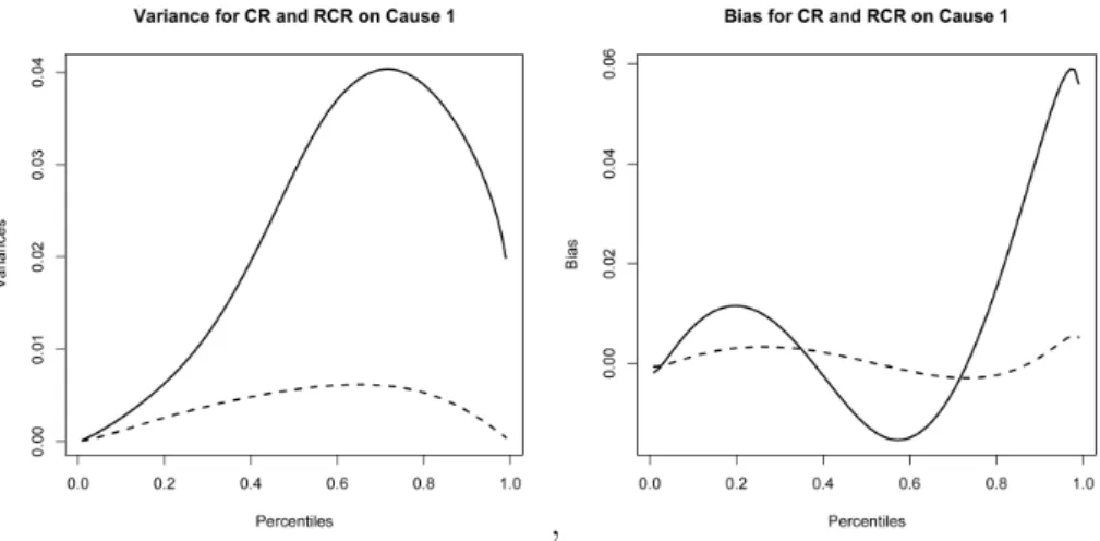
Figure 2 and Figure 3 show the simulated relative efficiency compar-ison between non-recurrent competing risks and recurrent competing risks under apartial repair modelwith two competing risks for the ponent lifetimes and the system lifetimes, respectively. For ease of com-parison, the simulated relative efficiencies were plotted as SCRM-based estimator relative to the RCRM-based estimator so that efficiencies are bounded by 1. Data sets with 30 systems were generated (N = 1000 replications) in order to estimate the parameters of the Weibull distri-butions so that 1000 estimates of the component lifetimes parameters were obtained. The estimated components lifetime distributions were evaluated at the 1st to the 99th percentiles. For each method, the bi-ases and variances of the component lifetime estimates were calculated for these percentiles and compared via their mean-squared error (MSE) to estimate the relative efficiencies. This process yielded the smoothed curves of Figure 2 and also of Figure 3. These curves are smooth since the same data sets were used to estimate the bias and variance, hence the MSE, at each of the percentiles. The system lifetime is plotted up to the 95th percentile associated with the Weibull(2,1/2) distribution of

Figure 2: Simulated relative efficiencies of the SCRM-based estimators relative to the RCRM-based estimators for the two component lifetime distributions under Weibull models for 30 systems based on N = 1000 simulation replications. The curves correspond to rates of the expo-nential distribution pertaining to the length of the monitoring period. These exponential rates are γ = 2,1,1/2,1/5, and 1/10, from top to bottom of figures.

Cause 1. Individual curves represent a different rate (2, 1, 1/2, 1/5, and 1/10, respectively from top to bottom) associated with an exponential censoring distribution. As the rate increases (which results in a decrease in the mean of the monitoring times), the simulated efficiency remains less than 1. When the rate increases, the mean of the censoring times eventually becomes less than the mean of both of the component lifetime distributions for the two risks which ultimately results in data sets that contain mostly censored observations for each of the 30 systems. There-fore, the resulting relative efficiencies become closer to unity. However, it is also interesting to note what happens when the rate associated with the exponential censoring distribution decreases, which increases the mean length of the monitoring period. When this occurs, the sim-ulated relative efficiency converges to 0, indicating that the increase in information gathered through repairing and recurring observations is highly beneficial. The interesting multi-peaked shapes of the curves can be attributed to the interplay between the variance curves of the esti-mates for the SCRM and RCRM scenarios as can be seen, for example, in Figure 4 which depicts these curves for the topmost curve of Figure 2 associated with an exponential censoring rate γ = 2. The simulated MSEs at the 10th percentile are 0.001170 and 0.00261, respectively for

Figure 3: Simulated relative efficiency of the SCRM-based system life-time estimator relative to the RCRM-based system lifelife-time estimator for the two component lifetime distributions under Weibull models for samples of size 30 based on N = 1000 simulation replications. The curves correspond to rates of the exponential distribution pertaining to the length of the monitoring period. These exponential rates are

γ = 2,1,1/2,1/5,and 1/10, from top to bottom of figures.

the RCRM and SCRM models, which yields a simulated relative effi-ciency of approximately 0.4485. Comparatively, the simulated variances at the 10th percentile are 0.001168 and 0.00255, respectively. Visual inspection reveals that as the difference between the variances increases in Figure 4 (with the largest difference being at approximately the 70th percentile), a corresponding change can be seen in the simulated relative efficiency which changes concavely at approximately the 70th percentile. The biases of the SCRM and RCRM estimates are also shown in Figure

4 but become essentially negligible in the MSEs since they get squared.

,

Figure 4: Variance and bias curves of the simulated estimates for the component lifetime distribution associated with F1(t) and with an

ex-ponential censoring rate of γ = 2. SCRM is depicted by a solid curve and RCRM by a dashed curve.

Overall, for the parameter values used in this simulation, there is a significant increase in efficiency of the RCRM-based estimator relative to the SCRM-based estimator. We expect that this efficiency behavior will also be the case for other parameter values, though more empirical investigations will be required especially for other distributional models.

5

Illustration Using Car Warranty Data

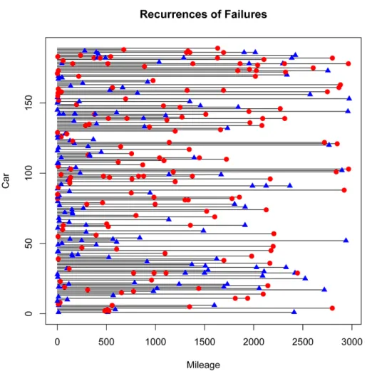
The time of failures (measured in mileage) for a sample of 189 cars under warranty were recorded together with the mode of failure (indicated by a 1 or 2). The circumstances of the data collection are not completely known to us, and it may be that this data suffers from selection bias, that is, only those cars that had warranty claims were in the sampled population. This will entail that the resulting estimates of the failure distributions based on this data set will tend to be stochastically smaller than the true failure time distributions of all the cars under warranty. This data, which was provided to us by Professor Ananda Sen of the University of Michigan, is pictured in Figure 5 with blue triangles repre-senting failures attributed to mode 1 and red circles denoting failures at-tributed to mode 2. In some cases, there were multiple failures recorded

at the same time. When this occurred, only the first recorded failure mode was used in the analysis. The final observation for each of these cars is a failure event. Thus, note that the actual data accrual does not exactly coincide with our model where the time to the end of monitoring is noninformative about the failure distributions. Additionally, the data possess discrete inter-event times. As such, caution should be observed in interpreting the results of this data illustration.

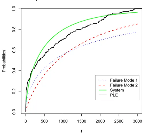
There were 153 failures attributed to failure mode 1 and 158 at-tributed to failure mode 2. The average (standard deviation) of observed miles between mode 1 failures was 675.1 (812.7) miles. Comparatively, failure mode 2 had an average (standard deviation) of observed miles between failures of 880.5 (800.8) miles. The data is modeled as partial repairs since typically car mechanics, but as we all know not always, only repair the failed components. Weibull distributions are assumed for the inter-event times for each of the failure modes. The estimates of the parameters are ˆα1 = 0.553, ˆβ1 = 1465.011, ˆα2 = 0.812, and

ˆ

β2 = 1351.176. Utilizing equation (3), estimates of the standard er-rors of these parameter estimates are obtained to be ˆse( ˆα1) = 0.040,

ˆ

se( ˆβ1) = 192.609, ˆse( ˆα2) = 0.059, and ˆse( ˆβ2) = 121.099. The

associ-ated marginal distribution curves and the system life distribution are depicted in Figure 6 for this data. Additionally, Figure 6 depicts the non-parametric estimator of the system life distribution based on the product limit estimators of the marginal distributions using only the first event (SCRM). Based on the discrepancies between the parametric estimator and the non-parametric estimator of the system life, we see that the Weibull assumption may not be an appropriate model for this data, providedthat the partial repair assumption is valid.

6

Simulation Studies

In order to demonstrate the small sample properties of our estimators, simulations that are similar to those for the efficiency comparisons were performed. However, the intent of these simulations was to demonstrate the properties of the estimation procedures for small samples. In these simulations we consider a system with three competing risks operating under partial repair with Weibull inter-event time distributions with dis-tinct parameters for each risk, (α1, β1), (α2, β2), and (α3, β3). For the

first and second simulations, 1000 data sets were simulated with n= 5 and n= 10 units, respectively, each operating under three partially re-paired Weibull causes of failure with θ = (α1 = 2, β1 = 2, α2 = 3, β2 =

Figure 5: Recurrences of two types of failure modes for 189 cars under warranty. Failure mode 1 = blue triangle, Failure mode 2 = red circle.

3, α3 = 4, β3 = 4). Censoring times were randomly generated from an exponential distribution with mean 4. Utilizing the constrOptim

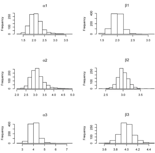
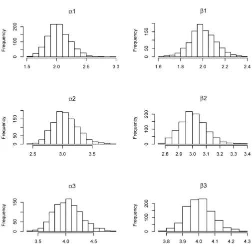
function in Rto minimize the negative log-likelihood, the estimates are obtained. The average estimate and standard error for the 1000 esti-mates are reported in Table 1 for n= 5 units and Table 2 for n = 10 units. Histograms of the parameter estimates are given in Figure 7 for the five units case and Figure 9 for the ten units case. There were on average, approximately 43, 65, and 86 observations of each of the three Weibull causes, respectively, for the five units case. Even with these relatively large number of observations per simulation, the estimated sampling distributions of the estimators for each of the parameters

Figure 6: Estimated inter-event time distributions for two types of fail-ure modes based on 189 cars under warranty.

hibit some skewness to the right for the shape parameters, α1,α2, and α3. This feature of the sampling distributions is more pronounced for the shape parameters’ estimates. With these sample sizes, the simulated sampling distributions of the scale parameters, β1, β2, and β3, are

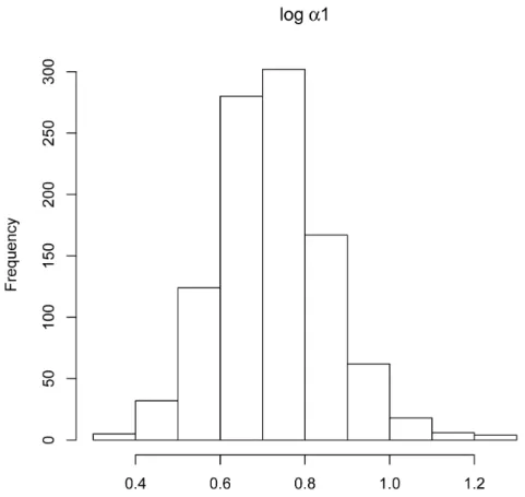
ap-proximately normal. A reviewer has suggested that a log-transformation of the estimates could improve the normal approximations to the sam-pling distributions. This suggestion is partly empirically validated by looking at Figure 8 which is the sampling distribution histogram of the logged estimates ofα1 from Figure 7. Utilizing the logged estimates may

become beneficial, for instance, when constructing confidence intervals for the parameter values through the use of the normal approximation to the sampling distribution.

When we increased to n= 10 units, the average number of observa-tions increased to approximately 88, 132, and 174 observaobserva-tions for each of the three Weibull causes, respectively. With this increase in the num-ber of observations, the simulated sampling distributions for the shape parameters, as well as the scale parameters, show approximately normal distributions.

Average Number of Estimated Parameter

True Events per Replication (Estimated Standard Error) Estimated Bias

α1= 2 43.184 2.082 (0.286) 0.082

β1= 2 1.996 (0.176) -0.004

α2= 3 64.943 3.096 (0.354) 0.096

β2= 3 2.997 (0.151) -0.003

α3= 4 85.984 4.072 (0.397) 0.072

β3= 4 4.002 (0.126) 0.002

Table 1: 1000 simulations of five units operating under three Weibull recurrent competing risks under a partial repair strategy and with a censoring mechanism generated by an exponential distribution with a mean of 4.

Average Number of Estimated Parameter

True Events per Replication (Estimated Standard Error) Estimated Bias

α1= 2 87.746 2.037 (0.187) 0.037

β1= 2 2.001 (0.116) 0.001

α2= 3 131.961 3.047 (0.213) 0.047

β2= 3 3.006 (0.097) 0.006

α3= 4 174.411 4.033 (0.247) 0.033

β3= 4 4.004 (0.083) 0.004

Table 2: 1000 simulations of 10 units operating under three Weibull recurrent competing risks under a partial repair strategy and with a censoring mechanism generated by an exponential distribution with a mean of 4.

To increase the number of observations for each cause, the mean of the censoring mechanism’s distribution and the number of units were increased to 6 and 50, respectively. The final simulation estimated the parameters for three partially repaired Weibull causes of failure withθ = (α1 = 2, β1= 2, α2 = 2.1, β2= 2.1, α3 = 2.2, β3= 2.2) for 50 units under an exponentially distributed censoring mechanism with mean 6. Again, there were 1000 simulation replications. Results from this simulation are shown in Table 3 and Figure 10. The simulated sampling distributions for the shape and scale parameters exhibit approximate normality.

Figure 7: Histogram of parameter estimates using α1 = 2, β1 = 2, α2 = 3, β2= 3, α3= 4,and β3= 4 for 1000 simulations of 5 units.

7

Concluding Remarks

This paper proposes a resource-efficient method for analyzing recurrent competing risks data. In particular, recurrent competing risks allow for a better use of the monitoring period by utilizing a repair strategy. Perfect and partial repair strategies were considered here. Other repair strategies not utilized in this paper offer alternative realistic applica-tions. For example, a minimal repair strategy would replace the failed component with another component of equivalent lifetime, which is an option when used parts are available. Given the resource-efficient nature of recurrent competing risks in which monitoring for more events contin-ues after a failure, it is not surprising that the recurrent competing risks method leads to more efficient estimation of the marginal distribution

Figure 8: Histogram of the logged parameter estimates of α1 depicted

in Figure 7.

functions of the component lifetimes, and consequently of the system life distribution, when compared to the non-recurrent competing risks model. The sampling distribution of the estimators are shown to be approximately normal distributions for large sample sizes. Simulation studies demonstrated the small (to moderate) sample properties of the estimators.

The methods were applied to a car warranty data to estimate the inter-event time distributions for the latent failure times. For the car warranty data, it was assumed that the failures occurred under Weibull marginal distributions, and under a partial repair strategy, aside from the independence of the latent time-to-event variables. A possibly more robust approach to the analysis of such types of recurrent competing risks data sets are through nonparametric methods where parametric assumptions are not imposed. Recent work on this has been done in [6],

Figure 9: Histogram of parameter estimates using α1 = 2, β1 = 2, α2 = 3, β2= 3, α3= 4,and β3= 4 for 1000 simulations of 10 units.

as well as in [16]. We also mention that a latent variable approach to the modeling of competing risks has its limitation as has been pointed out in [7, 10, 11, 17] among others. An important limitation, for instance, is that a competing risks data is insufficient to empirically verify the independence assumption among the latent failure-time variables, which could be a serious limitation in biomedical applications, but possibly may not be so serious for engineering and reliability applications. It will therefore be of interest to develop methods for dealing with recurrent competing risks data without using a latent variable approach and with possible dependencies among the different risks.

We close by noting that in a World where Time is Money and Money is Time, it is important to be considerate of both. When systems can

Average Number of Estimated Parameter

True Events per Replication (Estimated Standard Error) Estimated Bias

α1= 2.0 433.649 2.007 (0.077) 0.007

β1= 2.0 2.001 (0.049) 0.001

α2= 2.1 455.463 2.108 (0.074) 0.008

β2= 2.1 2.100 (0.049) 0.000

α3= 2.2 478.039 2.204 (0.079) 0.004

β3= 2.2 2.201 (0.050) 0.001

Table 3: 1000 simulations of 50 units operating under three Weibull recurrent competing risks under a partial repair strategy and with a censoring mechanism generated by an exponential distribution with a mean of 6.

Figure 10: Histogram of parameter estimates usingα1 = 2, β1 = 2, α2 = 2.1, β2 = 2.1, α3 = 2.2, β3 = 2.2 for 1000 simulations of 50 units.

be monitored for periods that extend beyond the first failure time, it is beneficial to allow systems to be repaired and to observe the

rences of failures over the monitoring period. So far, a limited amount of data has been collected in this manner so as to utilize information from recurrent events and competing risks. A data set that has been used in [12] concerns a recurrent competing risks setting under perfect repair by observing the failure of shunts due to multiple causes; see [4] for additional analysis of this data set. The analyses of this data set are first performed by ignoring the unique causes of failure and additionally using multiplicative regression models for each of the causes of failures to model three recurrences of shunt failures. However, we believe that it is now the right time that future studies and data collection should allow for recurrent competing risks to obtain more information, with a con-sequent beneficial result of producing more reliable conclusions, which will ultimately translate to better real-life decisions.

Acknowledgements

The authors would like to thank Professor Ananda Sen of the University of Michigan for providing the car warranty data and Professor Akim Adekpedjou of Missouri University of Science and Technology for his comments. They also thank Professor Jean-Yves Dauxois for inviting them to contribute to this special issue. The authors are also grateful to the reviewers for their highly constructive and pinpoint comments which considerably improved the paper.

References

[1] Abbring, J. H. and Van den Berg, G. J. (2003), The identifiability of the mixed proportional hazards competing risks model. J. Roy. Statist. Soc. Ser. B,65, 701–710.

[2] Bedford, T. and Lindqvist, B. H. (2004), The identifiability problem for repairable systems subject to competing risks. Adv. in Appl. Probab.,36(3), 774–790.

[3] Borgan, Ø. (1984), Maximum likelihood estimation in parametric counting process models, with applications to censored failure time data. Scand. J. Statist.,11(1), 1–16.

[4] Cook, R. J. and Lawless, J. F. (2007), The Statistical Analysis of Recurrent Events. Springer.

[5] Crowder, M. J. (2001), Classical Competing Risks. Chapman and Hall/CRC.

[6] Dauxois, J. Y. and Sencey, S. (2009), Non-parametric tests for recurrent events under competing risks. Scand. J. Statist., 36(4), 649–670.

[7] Heckman, J. J. and Honor´e, B. E. (1989), The identifiability of the competing risks model. Biometrika, 76(2), 325–330.

[8] Hollander, M. and Pe˜na, E. A. (2004), Nonparametric methods in reliability. Statist. Sci.,19(4), 644–651.

[9] Jacod, J. (1975), Multivariate point processes: predictable projec-tion, radon-nikodym derivatives, representation of martingales. Z. Wahrsch. verw. Geb., 34, 225–244.

[10] Kalbfleisch, J. D. and Prentice, R. L. (2002), The statistical analysis of failure time data. Wiley Series in Probability and Statistics, Wiley-Interscience, New Jeresy: John Wiley & Sons, second edition. [11] Lawless, J. F. (2003), Statistical models and methods for lifetime data. Wiley Series in Probability and Statistics, Wiley-Interscience, New Jeresy: John Wiley & Sons, second edition.

[12] Lawless, J. F., Wigg, M. B., Tuli, S., Drake, J., and Lamberti-Pasculli, M. (2001), Analysis of repeated failures of durations, with application to shunt failures for patients with paediatric hy-drocephalus. Applied Statistics, 50(4), 449–465.

[13] Lo, S. M. S. and Wilke, R. A. (2010), A copula model for dependent competing risks. Applied Statistics, 59(2), 359–376.

[14] Pe˜na, E. A., Strawderman, R. L., and Hollander, M. (2001), Non-parametric estimation with recurrent event data. J. Amer. Statist. Assoc.,96(456), 1299–1315.

[15] Serfling, R. (1980), Approximation Theorems of Mathematical Statistics. Wiley.

[16] Taylor, L. and Pe˜na, E. A. (2012), Nonparametric estimation with recurrent competing risks data. Technical report, Elon University. [17] Tsiatis, A. (1975), A nonidentifiability aspect of the problem of

competing risks. Proc. Nat. Acad. Sci. U.S.A.,72, 20–22.

[18] Tuli, S., Drake, J., Lawless, J. F., Wigg, M., and Lamberti-Pasculli, M. (1992), Risk factors for repeat cerebrospinal shunt failures in pediatric hydrocephalus. J. Neurosurgery, 31–38.

[19] Zheng, M. and Klein, J. P. (1995), Estimates of marginal sur-vival for dependent competing risks based on an assumed copula. Biometrika,82(1), 127–138.