I
NTRODUCTION TO THE
FINITE
ELEMENT
METHOD
G. P. Nikishkov
2004 Lecture Notes. University of Aizu, Aizu-Wakamatsu 965-8580, Japan [email protected]
2
Contents
1 Introduction 5
1.1 What is the finite element method . . . 5
1.2 How the FEM works . . . 5
1.3 Formulation of finite element equations . . . 6
1.3.1 Galerkin method . . . 6
1.3.2 Variational formulation . . . 8
2 Finite Element Equations for Heat Transfer 11 2.1 Problem Statement . . . 11
2.2 Finite element discretization of heat transfer equations . . . 12
2.3 Different Type Problems . . . 13
3 FEM for Solid Mechanics Problems 15 3.1 Problem statement . . . 15
3.2 Finite element equations . . . 16
3.3 Assembly of the global equation system . . . 18
4 Finite Elements 21 4.1 Two-dimensional triangular element . . . 21
4.2 Two-dimensional isoparametric elements . . . 22
4.2.1 Shape functions . . . 22
4.2.2 Strain-displacement matrix . . . 23
4.2.3 Element properties . . . 24
4.2.4 Integration in quadrilateral elements . . . 25
4.2.5 Calculation of strains and stresses . . . 26
4.3 Three-dimensional isoparametric elements . . . 28
4.3.1 Shape functions . . . 28
4.3.2 Strain-displacement matrix . . . 29
4.3.3 Element properties . . . 30
4.3.4 Efficient computation of the stiffness matrix . . . 30
4.3.5 Integration of the stiffness matrix . . . 31
4.3.6 Calculation of strains and stresses . . . 31
4.3.7 Extrapolation of strains and stresses . . . 31
4 CONTENTS
5 Discretization 33
5.1 Discrete model of the problem . . . 33
5.2 Mesh generation . . . 34
5.2.1 Mesh generators . . . 34
5.2.2 Mapping technique . . . 34
5.2.3 Delaunay triangulation . . . 36
6 Assembly and Solution 37 6.1 Disassembly and assembly . . . 37
6.2 Disassembly algorithm . . . 38
6.3 Assembly . . . 38
6.3.1 Assembly algorithm for vectors . . . 38
6.3.2 Assembly algorithm for matrices . . . 39
6.4 Displacement boundary conditions . . . 39
6.4.1 Explicit specification of displacement BC . . . 40
6.4.2 Method of large number . . . 40
6.5 Solution of Finite Element Equations . . . 40
6.5.1 Solution methods . . . 40
6.5.2 Direct LDU method with profile matrix . . . 41
6.5.3 Tuning of the LDU factorization . . . 43
Chapter 1
Introduction
1.1
What is the finite element method
The finite element method (FEM) is a numerical technique for solving problems which are described by partial differential equations or can be formulated as functional minimization. A domain of interest is represented as an assembly of finite elements. Approximating functions in finite elements are deter-mined in terms of nodal values of a physical field which is sought. A continuous physical problem is transformed into a discretized finite element problem with unknown nodal values. For a linear problem a system of linear algebraic equations should be solved. Values inside finite elements can be recovered using nodal values.
Two features of the FEM are worth to be mentioned:
1) Piece-wise approximation of physical fields on finite elements provides good precision even with simple approximating functions (increasing the number of elements we can achieve any precision). 2) Locality of approximation leads to sparse equation systems for a discretized problem. This helps to solve problems with very large number of nodal unknowns.
1.2
How the FEM works
To summarize in general terms how the finite element method works we list main steps of the finite element solution procedure below.
1. Discretize the continuum. The first step is to divide a solution region into finite elements. The finite element mesh is typically generated by a preprocessor program. The description of mesh consists of several arrays main of which are nodal coordinates and element connectivities.
2. Select interpolation functions. Interpolation functions are used to interpolate the field vari-ables over the element. Often, polynomials are selected as interpolation functions. The degree of the polynomial depends on the number of nodes assigned to the element.
3. Find the element properties. The matrix equation for the finite element should be established which relates the nodal values of the unknown function to other parameters. For this task different approaches can be used; the most convenient are: the variational approach and the Galerkin method.
4. Assemble the element equations. To find the global equation system for the whole solution region we must assemble all the element equations. In other words we must combine local element equations for all elements used for discretization. Element connectivities are used for the assembly process. Before solution, boundary conditions (which are not accounted in element equations) should be imposed.
6 CHAPTER 1. INTRODUCTION
1
2
3
0
L
2
L
x
x
x
1
x
2u
1
u
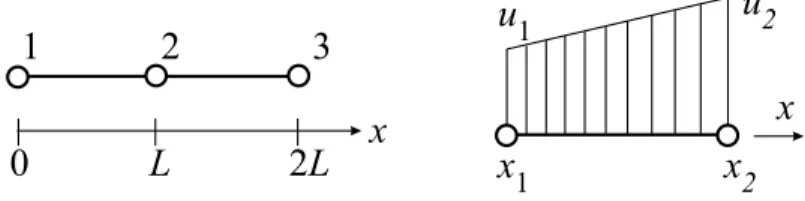
2Figure 1.1: Two one-dimensional linear elements and function interpolation inside element.
5. Solve the global equation system. The finite element global equation sytem is typically sparse, symmetric and positive definite. Direct and iterative methods can be used for solution. The nodal values of the sought function are produced as a result of the solution.
6. Compute additional results. In many cases we need to calculate additional parameters. For example, in mechanical problems strains and stresses are of interest in addition to displacements, which are obtained after solution of the global equation system.
1.3
Formulation of finite element equations
Several approaches can be used to transform the physical formulation of the problem to its finite element discrete analogue. If the physical formulation of the problem is known as a differential equation then the most popular method of its finite element formulation is the Galerkin method. If the physical problem can be formulated as minimization of a functional then variational formulation of the finite element equations is usually used.
1.3.1 Galerkin method
Let us use simple one-dimensional example for the explanation of finite element formulation using the Galerkin method. Suppose that we need to solve numerically the following differential equation:
ad
2u
dx2 +b= 0, 0≤x≤2L (1.1)
with boundary conditions
u|x=0= 0
adu
dx|x=2L=R
(1.2)
whereuis an unknown solution. We are going to solve the problem using two linear one-dimensional finite elements as shown in Fig. 1.1.
Fist, consider a finite element presented on the right of Figure. The element has two nodes and approximation of the functionu(x)can be done as follows:
u=N1u1+N2u2 = [N]{u}
[N] = [N1 N2]
{u}={u1 u2}
1.3. FORMULATION OF FINITE ELEMENT EQUATIONS 7
whereNi are the so called shape functions N1= 1− x−x1
x2−x1
N2= xx−x1 2−x1
(1.4)
which are used for interpolation ofu(x)using its nodal values. Nodal valuesu1 andu2 are unknowns
which should be determined from the discrete global equation system.
After substituting u expressed through its nodal values and shape functions, in the differential equation, it has the following approximate form:
a d2
dx2[N]{u}+b=ψ (1.5)
whereψis a nonzero residual because of approximate representation of a function inside a finite ele-ment. The Galerkin method provides residual minimization by multiplying terms of the above equation by shape functions, integrating over the element and equating to zero:
Z x2
x1
[N]Ta d
2
dx2[N]{u}dx+
Z x2
x1
[N]Tbdx= 0 (1.6)
Use of integration by parts leads to the following discrete form of the differential equation for the finite element:
Z x2
x1 · dN dx ¸T a · dN dx ¸
dx{u}−
Z x2
x1
[N]Tbdx−
(
0 1
)
adu
dx|x=x2+
(
1 0
)
adu
dx|x=x1 = 0 (1.7)
Usually such relation for a finite element is presented as:
[k]{u}={f}
[k] =
Z x2
x1 · dN dx ¸T a · dN dx ¸ dx
{f}=
Z x2
x1
[N]Tbdx+
(
0 1
)
adu
dx|x=x2 −
(
1 0
)
adu dx|x=x1
(1.8)
In solid mechanics[k]is called stiffness matrix and{f}is called load vector. In the considered simple case for two finite elements of lengthLstiffness matrices and the load vectors can be easily calculated:
[k1] = [k2] = a L
"
1 −1
−1 1
#
{f1}= bL2
(
1 1
)
, {f2}= bL2
( 1 1 ) + ( 0 R ) (1.9)
The above relations provide finite element equations for the two separate finite elements. A global equation system for the domain with 2 elements and 3 nodes can be obtained by an assembly of element equations. In our simple case it is clear that elements interact with each other at the node with global number 2. The assembled global equation system is:
a L
1 −1 0
−1 2 −1 0 −1 1
u1 u2 u3 = bL 2 1 2 1 + 0 0 R (1.10)
8 CHAPTER 1. INTRODUCTION
0.0 0.5 1.0 1.5 2.0 0 1 2 3 4
x
u
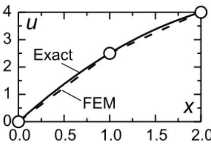
FEM ExactFigure 1.2: Comparison of finite element solution and exact solution.
After application of the boundary conditionu(x= 0) = 0the final appearance of the global equation system is: a L
1 0 0 0 2 −1 0 −1 1
u1 u2 u3 = bL 2 0 2 1 + 0 0 R (1.11)
Nodal valuesui are obtained as results of solution of linear algebraic equation system. The value of u at any point inside a finite element can be calculated using the shape functions. The finite element solution of the differential equation is shown in Fig. 1.2 fora= 1, b= 1, L= 1andR= 1.
Exact solution is a quadratic function. The finite element solution with the use of the simplest element is piece-wise linear. More precise finite element solution can be obtained increasing the number of simple elements or with the use of elements with more complicated shape functions. It is worth noting that at nodes the finite element method provides exact values ofu(just for this particular problem). Finite elements with linear shape functions produce exact nodal values if the sought solution is quadratic. Quadratic elements give exact nodal values for the cubic solution etc.
1.3.2 Variational formulation
The differential equation
ad2u
dx2 +b= 0, 0≤x≤2L
u|x=0= 0
adu
dx|x=2L=R
(1.12)
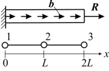
with a = EA has the following physical meaning in solid mechanics. It describes tension of the one dimensional bar with cross-sectional areaA made of material with the elasticity modulusE and subjected to a distributed loadband a concentrated loadRat its right end as shown in Fig 1.3.
Such problem can be formulated in terms of minimizing the potential energy functionalΠ:
Π = Z L 1 2a µ du dx ¶2 dx− Z
Lbudx−Ru|x=2L u|x=0= 0
1.3. FORMULATION OF FINITE ELEMENT EQUATIONS 9
1
2
3
0
L
2
L
x
R
b
Figure 1.3: Tension of the one dimensional bar subjected to a distributed load and a concentrated load.
Using representation of{u}with shape functions (1.3)-(1.4) we can write the value of potential energy for the second finite element as:
Πe=
Z x2
x1
1 2a{u}
T
·
dN dx
¸T·
dN dx
¸
{u}dx
−
Z x2
x1
{u}T[N]Tbdx− {u}T
(
0
R
) (1.14)
The condition for the minimum ofΠis:
δΠ = ∂Π
∂u1δu1+...+
∂Π
∂unδun= 0 (1.15)
which is equivalent to
∂Π
∂ui = 0, i= 1...n (1.16)
It is easy to check that differentiation ofΠin respect touigives the finite element equilibrium equation which is coincide with equation obtained by the Galerkin method:
Z x2
x1
·
dN dx
¸T
EA
·
dN dx
¸
dx{u}−
Z x2
x1
[N]Tbdx−
(
0
R
)
= 0 (1.17)
Example. Obtain shape functions for the one-dimensional quadratic element with three nodes. Use local coordinate system−1≤ξ≤1.
1
2
3
-1
0
1
x
Solution. With shape functions, any field inside element is presented as:
u(ξ) =XNiui , i= 1, 2, 3
At nodes the approximated function should be equal to its nodal value:
u(−1) =u1 u(0) =u2
10 CHAPTER 1. INTRODUCTION
Since the element has three nodes the shape functions can be quadratic polynomials (with three coeffi-cients). The shape functionN1can be written as:
N1 =α1+α2ξ+α3ξ2
Unknown coefficientsαiare defined from the following system of equations: N1(−1) =α1−α2+α3 = 1
N1(0) =α1 = 0
N1(1) =α1+α2+α3 = 0
The solution is:α1= 0, α2=−1/2, α3= 1/2. Thus the shape function N1is equal to:
N1 =−12ξ(1−ξ)
Similarly it is possible to obtain that the shape functionsN2andN3are equal to:
N2= 1−ξ2 N3= 12ξ(1 +ξ)
Chapter 2
Finite Element Equations for Heat
Transfer
2.1
Problem Statement
Let us consider an isotropic body with temperature dependent heat transfer. A basic equation of heat transfer has the following appearance:
−
µ
∂qx ∂x +
∂qy ∂y +
∂qz ∂z
+Q=ρc∂T
∂t (2.1)
Hereqx, qy andqz are components of heat flow through the unit area; Q = Q(x, y, z, t)is the inner heat generation rate per unit volume;ρis material density;cis heat capacity;T is temperature andtis time. According to the Fourier’s law the components of heat flow can be expressed as follows:
qx=−k∂T∂x qy =−k∂T∂y qz =−k∂T∂z
(2.2)
wherekis the thermal conductivity coefficient of the media. Substitution of Fourier’s relations gives the following basic heat transfer equation:
∂ ∂x
µ
k∂T ∂x
+ ∂
∂y
µ
k∂T ∂y
+ ∂
∂z
µ
k∂T ∂z
+Q=ρc∂T
∂t (2.3)
It is assumed that boundary conditions can be of the following types:
1. Specified temperature
Ts=T(x, y, z, t)onS1
2. Specified heat flow
qxnx+qyny+qznz=−qsonS2
3. Convection boundary conditions
12 CHAPTER 2. FINITE ELEMENT EQUATIONS FOR HEAT TRANSFER
qxnx+qyny+qznz=h(Ts−Te)onS3
whereh is the convection coefficient,Tsis an unknown surface temperature andTe is a known envi-ronmental temperature.
4. Radiation
qxnx+qyny+qznz=σεTs4−αqronS4
whereσis the Stefan-Boltzmann constant;εis the surface emission coefficient;αis the surface absorp-tion coefficient andqris incoming heat flow per unit surface area.
For transient problems it is necessary to specify a temperature field for a body at the timet= 0:
T(x, y, z,0) =T0(x, y, z) (2.4)
2.2
Finite element discretization of heat transfer equations
A domainV is divided into finite elements connected at nodes. We are going to write all relations for a finite element. Global equations for the domain can be assembled from finite element equations using connectivity information.
Shape functionsNi are used for interpolation of temperature inside a finite element: T = [N]{T}
[N] = [ N1 N2 ... ]
{T}={ T1 T2 ... }
(2.5)
Differentiation of the temperature interpolation equation gives the following interpolation relation for temperature gradients:
∂T /∂x ∂T /∂y ∂T /∂z
=
∂N1/∂x ∂N2/∂x ...
∂N1/∂y ∂N2/∂y ...
∂N1/∂z ∂N2/∂z ...
{T}= [B]{T} (2.6)
Here{T}is a vector of temperatures at nodes;[N]is a matrix of shape functions and[B]is a matrix for temperature gradients interpolation.
Using Galerkin method, we can rewrite the basic heat transfer equation in the following form:
Z
V
µ
∂qx ∂x +
∂qy ∂y +
∂qz
∂z −Q+ρc ∂T
∂t
NidV = 0 (2.7)
Applying the divergence theorem to the first three terms, we arrive to the relations:
Z
V ρc∂T
∂tNidV −
Z
V
·
∂Ni ∂x
∂Ni ∂y
∂Ni ∂z
¸
{q}dV
=
Z
V
QNidV −
Z
S
{q}T{n}NidS
{q}T = [ qx qy qz ] {n}T = [ nx ny nz ]
2.3. DIFFERENT TYPE PROBLEMS 13
where{n}is an outer normal to the surface of the body. After insertion of boundary conditions into the above equation, the discretized equations are as follows:
Z
V ρc∂T
∂tNidV −
Z
V
·
∂Ni ∂x
∂Ni ∂y
∂Ni ∂z
¸
{q}dV
=
Z
V
QNidV −
Z
S1
{q}T{n}NidS
+
Z
S2
qsNidS−
Z
S3
h(T −Te)NidS−
Z
S4
(σεT4−αqr)NidS
(2.9)
It is worth noting that
{q}=−k[B]{T} (2.10)
The discretized finite element equations for heat transfer problems have the following finite form:
[C]{T˙}+ ([Kc] + [Kh] + [Kr]){T}
={RT}+{RQ}+{Rq}+{Rh}+{Rr} (2.11)
[C] =
Z
V
ρc[N]T[N]dV
[Kc] =
Z
V
k[B]T[B]dV
[Kh] =
Z
S3
h[N]T[N]dS
[Kr]{T}=
Z
S4
σεT4[N]dS
[RT] =−
Z
S1
{q}T{n}[N]TdS
[RQ] =
Z
V
Q[N]TdV
[Rq] =−
Z
S2
qs[N]TdS
[Rh] =−
Z
S3
hTe[N]TdS
[Rr] =−
Z
S4
αqr[N]TdS
(2.12)
2.3
Different Type Problems
Equations for different type problems can be deducted from the above general equation :
Stationary linear problem
14 CHAPTER 2. FINITE ELEMENT EQUATIONS FOR HEAT TRANSFER
Stationary nonlinear problem
([Kc] + [Kh] + [Kr]){T}
={RQ(T)}+{Rq(T)}+{Rh(T)}+{Rr(T)} (2.14) Transient linear problem
[C]{T˙(t)}+ ([Kc] + [Kh(t)]){T(t)}
={RQ(t)}+{Rq(t)}+{Rh(t)} (2.15) Transient nonlinear problem
[C(T)]{T˙}+ ([Kc(T)] + [Kh(T, t)] + [Kr(T)]){T}
Chapter 3
FEM for Solid Mechanics Problems
3.1
Problem statement
Let us consider a three-dimensional elastic body subjected to surface and body forces and temperature field. In addition, displacements are specified on some surface area. For given geometry of the body, applied loads, displacement boundary conditions, temperature field and material stress-strain law, it is necessary to determine the displacement field for the body. The corresponding strains and stresses are also of interest.
The displacements along coordinate axesx,yandzare defined by the displacement vector{u}:
{u}={u v w} (3.1)
Six different strain components can be placed in the strain vector{ε}:
{ε}={εx εy εz γxy γyz γzx} (3.2) For small strains the relationship between strains and displacements is:
{ε}= [D]{u} (3.3)
where[D]is the matrix differentiation operator:
[D] =
∂/∂x 0 0
0 ∂/∂y 0 0 0 ∂/∂z ∂/∂y ∂/∂x 0
0 ∂/∂z ∂/∂y
∂/∂z 0 ∂/∂x
(3.4)
Six different stress components are formed the stress vector{σ}:
{σ}={σx σy σz τxy τyz τzx} (3.5) which are related to strains for elastic body by the Hook’s law:
{σ}= [E]{εe}= [E]({ε} − {εt})
{εt}={αT αT αT 0 0 0} (3.6)
16 CHAPTER 3. FEM FOR SOLID MECHANICS PROBLEMS
Here{εe}is the elastic part of strains;{εt}is the thermal part of strains;αis the coefficient of thermal expansion;T is temperature. The elasticity matrix[E]has the following appearance:
[E] =
λ+ 2µ λ λ 0 0 0
λ λ+ 2µ λ 0 0 0
λ λ λ+ 2µ 0 0 0 0 0 0 µ 0 0 0 0 0 0 µ 0 0 0 0 0 0 µ
(3.7)
whereλandµare elastic Lame constants which can be expressed through the elasticity modulusEand Poisson’s ratioν:
λ= νE
(1 +ν)(1−2ν)
µ= E
2(1 +ν)
(3.8)
The purpose of finite element solution of elastic problem is to find such displacement field which provides minimum to the functional of total potential energyΠ:
Π =
Z
V
1 2{ε
e}T{σ}dv−
Z
V {u}
T{pV}dV −
Z
S{u}
T{pS}dS (3.9)
Here{pV} = {pVx pVy pVz} is the vector of body force and{pS} = {pxS pSy pSz} is the vector of surface force. Prescribed displacements are specified on the part of body surface where surface forces are absent.
Displacement boundary conditions are not present in the functional ofΠ. Because of these, dis-placement boundary conditions should be implemented after assembly of finite element equations.
3.2
Finite element equations
Let us consider some abstract three-dimensional finite element having the vector of nodal displacements {q}:
{q}={u1 v1 w1 u2 v2 w2 ...} (3.10) Displacements at some point inside a finite element{u}can be determined with the use of nodal dis-placements{q}and shape functionsNi:
u=PNiui v=PNivi w=PNiwi
(3.11)
These relations can be rewritten in a matrix form as follows:
{u}= [N]{q}
[N] =
N1 0 0 N2 ...
0 N1 0 0 ...
0 0 N1 0 ...
3.2. FINITE ELEMENT EQUATIONS 17
Strains can also be determined through displacements at nodal points:
{ε}= [B]{q}
[B] = [D][N] = [B1 B2 B3 ...] (3.13)
Matrix[B]is called the displacement differentiation matrix. It can be obtained by differentiation of displacements expressed through shape functions and nodal displacements:
[Bi] =
∂Ni/∂x 0 0
0 ∂Ni/∂y 0
0 0 ∂Ni/∂z ∂Ni/∂y ∂Ni/∂x 0
0 ∂Ni/∂z ∂Ni/∂y ∂Ni/∂z 0 ∂Ni/∂x
(3.14)
Now using relations for stresses and strains we are able to express the total potential energy through nodal displacements:
Π =
Z
V
1
2([B]{q} − {ε
t})T[E]([B]{q} − {εt})dV −
Z
V ([N]{q})
T{pV}dV −
Z
S([N]{q})
T{pS}dS (3.15)
Nodal displacements{q}which correspond to the minimum of the functionalΠare determined by the conditions:
½
∂Π
∂q
¾
= 0 (3.16)
Differentiation ofΠin respect to nodal displacements{q}produces the following equilibrium equations for a finite element:
Z
V [B]
T[E][B]dV{q} −Z V [B]
T[E]{εt}dV −
Z
V [N]
T{pV}dV −Z S[N]
T{pS}dS= 0 (3.17)
which is usually presented in the following form:
[k]{q}={f} {f}={p}+{h}
[k] =
Z
V [B]
T[E][B]dV {p}=
Z
V [N]
T{pV}dV +
Z
S[N]
T{pS}dS {h}=
Z
V [B]
T[E]{εt}dV
(3.18)
Here[k]is the element stiffness matrix;{f}is the load vector; {p}is the vector of actual forces and {h}is the thermal vector which represents fictitious forces for modeling thermal expansion.
18 CHAPTER 3. FEM FOR SOLID MECHANICS PROBLEMS
3.3
Assembly of the global equation system
The aim of assembly is to form the global equation system
[K]{Q}={F} (3.19)
using element equations
[ki]{qi}={fi} (3.20)
Here[ki], [qi]and[fi]are the stiffness matrix, the displacement vector and the load vector of the ith finite element;[K],{Q}and{F}are global stiffness matrix, displacement vector and load vector.
In order to derive an assembly algorithm let us present the total potential energy for the body as a sum of element potential energiesπi:
Π =Xπi =
X1
2{qi}
T[k
i]{qi} −
X
{qi}T{fi}+
X
Ei0 (3.21)
whereEi0 is the fraction of potential energy related to free thermal expansion:
Ei0 =
Z
Vi
1 2{ε
t}T[E]{εt}dV (3.22)
Let us introduce the following vectors and a matrix where element vectors and matrices are simply placed:
{Qd}={{q1} {q2}
{Fd}={{f1} {f2}...} (3.23)
[Kd] =
[k1] 0 0
0 [k2] 0
0 0 ...
(3.24)
It is evident that it is easy to find matrix[A]such that {Qd}= [A]{Q}
{Fd}= [A]{F} (3.25)
The total potential energy for the body can be rewritten in the following form:
Π = 1 2{Qd}
T[K
d]{Qd} − {Qd}T{Fd}+
X
Ei0
= 1 2{Q}
T[A]T[K
d][A]{Q} − {Q}T[A]T{Fd}+
X
Ei0 (3.26)
Using the condition of minimum of the total potential energy
½
∂Π
∂Q
¾
= 0 (3.27)
we arrive at the following global equation system:
3.3. ASSEMBLY OF THE GLOBAL EQUATION SYSTEM 19
The last equation shows that algorithms of assembly the global stiffness matrix and the global load vector are:
[K] = [A]T[Kd][A]
{F}= [A]T{Fd} (3.29)
Here[A]is the matrix providing transformation from global to local enumeration. Fraction of nonzero (unit) entries in the matrix[A]is very small. Because of this the matrix[A]is never used explicitly in actual computer codes.
Example. Write down a matrix[A], which relates local (element) and global (domain) node numbers for the following finite element mesh:
1
4 5 6
2 3 1 2 7 8 3 1 2 3 4 Node order for an element
Solution. To make the matrix representation compact let us assume that each node has one degree of freedom (note that in three-dimensional solid mechanics problem there are three degrees of freedom at each node). The matrix[A]relates element and global nodal values in the following way:
{Qd}= [A]{Q}
where {Q} is a global vector of nodal values and {Qd} is vector containing element vectors. The explicit rewriting of the above relation looks as follows:
Q1 Q2 Q5 Q4 Q2 Q3 Q6 Q5 Q5 Q6 Q8 Q7 =
1 0 0 0 0 0 0 0 0 1 0 0 0 0 0 0 0 0 0 0 1 0 0 0 0 0 0 1 0 0 0 0 0 1 0 0 0 0 0 0 0 0 1 0 0 0 0 0 0 0 0 0 0 1 0 0 0 0 0 0 1 0 0 0 0 0 0 0 1 0 0 0 0 0 0 0 0 1 0 0 0 0 0 0 0 0 0 1 0 0 0 0 0 0 1 0
Q1 Q2 Q3 Q4 Q5 Q6 Q7 Q8
Chapter 4
Finite Elements
4.1
Two-dimensional triangular element
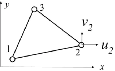
Triangular finite element was the first finite element proposed for continuous problems. Because of simplicity it can be used as an introduction to other elements. A triangular finite element in the co-ordinate systemxy is shown in Fig. 4.1. Since the element has three nodes, linear approximation of displacementsuandvis selected:
u(x, y) =N1u1+N2u2+N3u3
v(x, y) =N1v1+N2v2+N3v3
Ni=αi+βix+γiy
(4.1)
Shape functionsNi(x, y)can be determined from the following equation system:
u(xi, yi) =ui , i= 1, 2, 3 (4.2) Shape functions for the triangular element can be presented as:
Ni= 2∆1 (ai+bix+ciy) ai =xi+1yi+2−xi+2yi+1
bi=yi+1−yi+2
ci=xi+2−xi+1
∆ = 1
2(x2y3+x3y1+x1y2−x2y1−x3y2−x1y3)
(4.3)
1
2
3
x
y
u
2
v
2
Figure 4.1: Triangular finite element is the simplest two-dimensional element.
22 CHAPTER 4. FINITE ELEMENTS
where∆is the element area. The matrix[B]for interpolating strains using nodal displacements is equal to:
[B] = 1 2∆
b1 0 b2 0 b3 0
0 c1 0 c2 0 c3
c1 b1 c2 b2 c3 b3
(4.4)
The elasticity matrix[E]has the following appearance for plane problems:
[E] =
λ+ 2µ λ 0
λ λ+ 2µ 0 0 0 µ
(4.5)
whereλandµare Lame constants:
λ= νE
(1 +ν)(1−2ν) for plane strain
λ= νE
1−ν2 for plane stress
µ= E
2(1 +ν)
(4.6)
HereEis the elasticity modulus andνis the Poisson’s ratio.
The stiffness matrix for the three-node triangular element can be calculated as:
[k] =
Z
V [B]
T[E][B]dV = [B]T[E][B]∆ (4.7) Here it was taken into account that both matrices [B]and[E]do not depend on coordinates. It was assumed that the element has unit thickness. Since the matrix[B]is constant inside the element the strains and stresses are also constant inside the triangular element.
4.2
Two-dimensional isoparametric elements
Isoparametric finite elements are based on the parametric definition of both coordinate and displacement functions. The same shape functions are used for specification of the element shape and for interpolation of the displacement field.
4.2.1 Shape functions
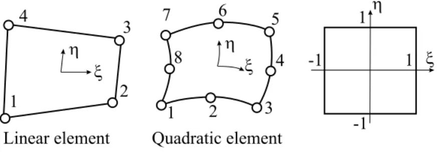
Linear and quadratic two-dimensional isoparametric finite elements are presented in Figure 4.2. Shape functionsNi are defined in local coordinatesξ, η (−1 ≤ ξ, η ≤ 1). The same shape functions are used for interpolations of displacements and coordinates:
u=PNiui , v=PNivi
x=PNixi, y=PNiyi (4.8)
whereu,vare displacement components at point with local coordinates(ξ, η);ui,vi are displacement values at the nodes of the finite element;x,yare point coordinates andxi,yiare coordinates of element nodes. Matrix form of the above relations is as follows:
{u}= [N]{q} {u}={u v}
{q}={u1 v1u2v2 ...}
4.2. TWO-DIMENSIONAL ISOPARAMETRIC ELEMENTS 23
1
3
x
4
2
h
x h
1 2 3
4 5 6
7
8 x
h
1 1 -1
-1 Linear element Quadratic element
Figure 4.2: Linear and quadratic finite elements and their representation in the local coordinate system.
{x}= [N]{xe} {x}={x y}
{xe}={x1 y1 x2 y2...}
(4.10)
where the interpolation matrix for nodal values is:
[N] =
"
N1 0 N2 0 ...
0 N1 0 N2 ...
#
(4.11)
Shape functions for linear and quadratic two-dimensional isoparametric elements are given by: linear element (4 nodes):
Ni = 14(1 +ξ0)(1 +η0) (4.12)
quadratic element (8 nodes):
Ni= 14(1 +ξ0)(1 +η0)− 14(1−ξ2)(1 +η0)
−1
4(1 +ξ0)(1−η
2) i= 1, 3, 5, 7
Ni= 12(1−ξ2)(1 +η0), i= 2, 6
Ni= 12(1 +ξ0)(1−η2), i= 4, 8
(4.13)
In the above equations the following notation is used: ξ0 =ξξi , η0 =ηηi whereξi,ηi are values of local coordinatesξ,ηat nodes.
4.2.2 Strain-displacement matrix
For plane problem the strain vector contains three components:
{ε}={εx εy γxy}=
½
∂u ∂x
∂v ∂y
∂v ∂x+
∂u ∂y
¾
24 CHAPTER 4. FINITE ELEMENTS
The strain-displacement matrix which is employed to compute strains at any point inside the element using nodal displacements is:
[B] = [B1B2...]
[Bi] =
∂Ni ∂x 0
0 ∂Ni
∂y ∂Ni ∂y ∂Ni ∂x (4.15)
While shape functions are expressed through the local coordinatesξ,ηthe strain-displacement matrix contains derivatives in respect to the global coordinatesx,y. Derivatives can be easily converted from one coordinate system to the other by means of the chain rule of partial differentiation:
∂Ni ∂ξ ∂Ni ∂η = ∂x ∂ξ ∂y ∂ξ ∂x ∂η ∂y ∂η ∂Ni ∂x ∂Ni ∂y
= [J]
∂Ni ∂x ∂Ni ∂y (4.16)
where[J]is the Jacobian matrix. The derivatives in respect to the global coordinates are computed with the use of inverse of the Jacobian matrix:
∂Ni ∂x ∂Ni ∂y
= [J]−1
∂Ni ∂ξ ∂Ni ∂η (4.17)
The components of the Jacobian matrix are calculated using derivatives of shape functionsNiin respect to the local coordinatesξ,ηand global coordinates of element nodesxi,yi:
∂x ∂ξ =
X∂Ni
∂ξ xi , ∂x ∂η =
X∂Ni
∂η xi ∂y
∂ξ =
X∂Ni
∂ξ yi , ∂y ∂η =
X∂Ni
∂η yi
(4.18)
The determinant of the Jacobian matrix|J|is used for the transformation of integrals from the global coordinate system to the local coordinate system:
dV =dxdy=|J|dξdη (4.19)
4.2.3 Element properties
Element matrices and vectors are calculated as follows:
stiffness matrix
[k] =
Z
V [B]
T[E][B]dV (4.20)
force vector (volume and surface loads)
{p}=
Z
V [N]
T{pV}dV +
Z
S[N]
4.2. TWO-DIMENSIONAL ISOPARAMETRIC ELEMENTS 25
thermal vector (fictitious forces to simulate thermal expansion)
{h}=
Z
V [B]
T[E]{εt}dV (4.22)
The elasticity matrix[E]is given by relation (4.5).
4.2.4 Integration in quadrilateral elements
Integration of expressions for stiffness matrices and load vectors can not be performed analytically for general case of isoparametric elements. Instead, stiffness matrices and load vectors are typically evalu-ated numerically using Gauss quadrature over quadrilateral regions. The Gauss quadrature formula for the volume integral in two-dimensional case is of the form:
I =
Z 1
−1
Z 1
−1f(ξ, η)dξdη=
n X i=1 n X j=1
f(ξi, ηj)wiwj (4.23)
whereξi, ηj are abscissae andwi are weighting coefficients of the Gauss integration rule. Abscissae and weights of Gauss quadrature forn= 1,2,3 are given in Table:
Abscissae and weights of Gauss quadrature
n ξi wi
1 0 2
2 ∓1/√3 1
3 0 8/9
∓p3/5 5/9
To compute the nodal equivalent of the surface load, the surface integral is replaced by line integration along element side. The fraction of the surface load is evaluated as:
{p}=
Z
S[N]
T{pS}dS=
Z 1
−1[N]
T{pS}ds
dξdξ (4.24)
ds dξ = sµ dx dξ ¶2 + µ dy dξ ¶2 (4.25)
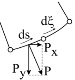
Heresis a global coordinate along the element side andξis a local coordinate along the element side. If the distributed load load is applied along the normal to the element side as shown in Fig. 4.3 then the nodal equivalent of such load is:
{p}=RS[N]Tp
dy ds −dx ds ds dξdξ=
R1
−1[N]Tp
dy dξ −dx dξ dξ (4.26)
Example. Calculate nodal equivalents of a distributed load with constant intensity applied to the side of a two-dimensional quadratic element:
26 CHAPTER 4. FINITE ELEMENTS
d
x
ds
P
Px
Py
Figure 4.3: Distributed normal load on a side of a quadratic element.
1
2
3
-1
0
1
x
p
=1
x
l=1
Solution. The nodal equivalent of the distributed load is calculated as:
{p}=
Z 1
−1[N]
Tpdx dξdξ
or
{p}=
p1 p2 p3 = Z 1 −1 N1 N2 N3 p dx dξdξ, dx dξ = 1 2
The shape functions for the one-dimensional quadratic element are:
N1 =−1
2ξ(1−ξ), N2 = 1−ξ
2, N
3 =
1
2ξ(1 +ξ)
The values of nodal forces at nodes 1, 2 and 3 are defined by integration:
p1 =−
Z 1
−1
1
2ξ(1−ξ) 1 2dξ=
1 6
p2 =
Z 1
−1(1−ξ 2)1
2dξ= 2 3
p3 =
Z 1
−1
1
2ξ(1 +ξ) 1 2dξ=
1 6
The example shows that physical approach cannot be used for the estimation of nodal equivalents of a distributed load. It works for linear elements; however, it does not work for more complicated elements.
4.2.5 Calculation of strains and stresses
Strains at any point an element are determined using Cauchy relations (4.14) with the use of the dis-placement differentiation matrix (4.15):
4.2. TWO-DIMENSIONAL ISOPARAMETRIC ELEMENTS 27
1 2
3 4
x h
(2) (1)
(4) (3)
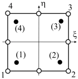
Figure 4.4: Numbering of integration points and vertices for the 8-node isoparametric element.
Stresses are calculated with the Hook’s law:
{σ}= [E]{εe}= [E]({ε} − {εt}) (4.28)
where{εt}is the vector of free thermal expansion:
{εt}={αT αT 0} (4.29)
Precision of strains and stresses is significantly dependent on the point location where they are com-puted. The highest precision for displacement gradients are at the geometric center for the linear ele-ment and at reduced integration points2×2for the quadratic quadrilateral element.
For quadratic elements with 8 nodes, strains and stresses have best precision at2×2integration points with local coordinates ξ, η = ±1/√3. A possible way to create continuous stress field with reasonable accuracy consists of: 1) extrapolation of stresses from reduced integration points to nodes; 2) averaging contributions from finite elements at all nodes of the finite element model. Later stresses can be interpolated from nodes using quadratic shape functions.
Let us consider quadratic element in the local coordinate systemξ, ηas shown in Fig. 4.4 where integration points are numbered as (1)...(4); corner nodes have numbers 1...4. For extrapolation (inside quadratic element) we are going to employ linear shape functions. In matrix form the extrapolation relation can be presented as follows:
fi =Li(m)f(m) (4.30)
where f(m) are known function values at reduces integration points; fi are function values at vertex nodes andLi(m)is the symmetric extrapolation matrix:
Li(m)=
A B C B A B C A B A
A= 1 +
√
3 2
B=−1
2
C= 1 +
√
3 2
28 CHAPTER 4. FINITE ELEMENTS
1
3 4
2 1 2 3 4
5 6
7 8
x
h
Linear element
Quadratic element
5
6 7 8
9 10
11 12
13 14 15 16 17
18 19 20
z
Figure 4.5: Linear and quadratic three-dimensional finite elements and their representation in the local coordinate system.
4.3
Three-dimensional isoparametric elements
4.3.1 Shape functions
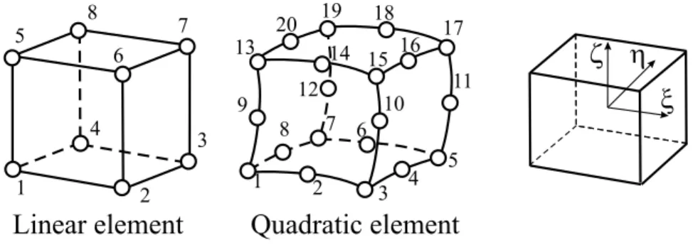
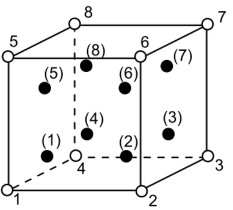
Hexahedral (or brick-type) linear 8-node and quadratic 20-node three-dimensional isoparametric ele-ments are depicted in Fig. 4.5. The term ”isoparametric” means that geometry and displacement field are specified in parametric form and are interpolated with the same functions. Shape functions used for interpolation are polynomials of the local coordinatesξ,ηandζ (−1≤ξ, η, ζ ≤1). Both coordinates and displacements are interpolated with the same shape functions:
{u}= [N]{q} {u}={u v w}
{q}={u1 v1w1 u2 v2w2 ...}
(4.32)
{x}= [N]{xe} {x}={x y z}
{xe}={x1 y1 z1 x2 y2 z2 ...}
(4.33)
Hereu, v, ware displacements at point with local coordinatesξ, η, ζ;ui, vi, wiare displacement values at nodes; x, y, z are point coordinates and xi, yi, zi are coordinates of nodes. The matrix of shape functions is:
[N] =
N1 0 0 N2 0 0 ...
0 N1 0 0 N2 0 ...
0 0 N1 0 0 N2 ...
(4.34)
Shape functions of the linear element are equal to:
Ni= 1
8(1 +ξ0)(1 +η0)(1 +ς0)
ξ0=ξξi, η0 =ηηi, ς0=ςςi
4.3. THREE-DIMENSIONAL ISOPARAMETRIC ELEMENTS 29
For the quadratic element with 20 nodes the shape functions can be written in the following form:
Ni= 18(1 +ξ0)(1 +η0)(1 +ς0)(ξ0+η0+ς0−2) vertices
Ni= 14(1−ξ2)(1 +η0)(1 +ς0), i= 2, 6, 14, 18
Ni=
1 4(1−η
2)(1 +ξ
0)(1 +ς0), i= 4, 8, 16, 20
Ni= 1 4(1−ς
2)(1 +ξ
0)(1 +η0), i= 9, 10, 11, 12
(4.36)
In the above relationsξi,ηi,ζiare values of local coordinatesξ,η,ζat nodes.
4.3.2 Strain-displacement matrix
The strain vector{ε}contains six different components of the strain tensor:
{ε}={εx εy εz γxy γyz γzx} (4.37) The strain-displacement matrix for three-dimensional elements has the following appearance:
[B] = [D][N] = [B1 B2 B3 ...] (4.38)
[Bi] =
∂Ni/∂x 0 0
0 ∂Ni/∂y 0
0 0 ∂Ni/∂z ∂Ni/∂y ∂Ni/∂x 0
0 ∂Ni/∂z ∂Ni/∂y ∂Ni/∂z 0 ∂Ni/∂x
(4.39)
Derivatives of shape functions in respect to global coordinates are obtained as follows:
∂Ni/∂x ∂Ni/∂y ∂Ni/∂z
= [J]
−1
∂Ni/∂ξ ∂Ni/∂η ∂Ni/∂ς
(4.40)
where the Jacobian matrix has the appearance:
[J] =
∂x/∂ξ ∂y/∂ξ ∂z/∂ξ ∂x/∂η ∂y/∂η ∂z/∂η ∂x/∂ς ∂y/∂ς ∂z/∂ς
(4.41)
The partial derivatives of x, y, z in respect to ξ, η,ζ are found by differentiation of displacements expressed through shape functions and nodal displacement values:
∂x ∂ξ =
X∂Ni
∂ξ xi , ∂x ∂η =
X∂Ni
∂η xi , ∂x ∂ζ =
X∂Ni
∂ζ xi ∂y
∂ξ =
X∂Ni
∂ξ yi , ∂y ∂η =
X∂Ni
∂η yi , ∂y ∂ζ =
X∂Ni
∂ζ yi ∂z
∂ξ =
X∂Ni
∂ξ zi , ∂z ∂η =
X∂Ni
∂η zi , ∂z ∂ζ =
X∂Ni
∂ζ zi
(4.42)
The transformation of integrals from the global coordinate system to the local coordinate system is performed with the use of determinant of the Jacobian matrix:
30 CHAPTER 4. FINITE ELEMENTS
4.3.3 Element properties
Element equilibrium equation has the following form:
[k]{q}={f}
{f}={p}+{h} (4.44)
Element matrices and vectors are:
stiffness matrix
[k] =
Z
V [B]
T[E][B]dV (4.45)
force vector (volume and surface loads)
{p}=
Z
V [N]
T{pV}dV +Z S[N]
T{pS}dS (4.46)
thermal vector (fictitious forces to simulate thermal expansion)
{h}=
Z
V [B]
T[E]{εt}dV (4.47)
The elasticity matrix[E]is:
[E] =
λ+ 2µ λ λ 0 0 0
λ λ+ 2µ λ 0 0 0
λ λ λ+ 2µ 0 0 0 0 0 0 µ 0 0 0 0 0 0 µ 0 0 0 0 0 0 µ
(4.48)
whereλandµare elastic Lame constants which can be expressed through the elasticity modulusEand Poisson’s ratioν:
λ= νE
(1 +ν)(1−2ν)
µ= E
2(1 +ν)
(4.49)
4.3.4 Efficient computation of the stiffness matrix
Calculation of the element stiffness matrix by multiplication of three matrices involves many arithmetic operations with zeros. After performing multiplications in closed form, coefficients of the element stiffness matrix[k]can be expressed as follows:
kiimn=
Z
V
·
β∂Nm ∂xi
∂Nn ∂xi +µ
µ
∂Nm ∂xi+1
∂Nm ∂xi+1 +
∂Nm ∂xi+2
∂Nm ∂xi+2
¶¸
dV kijmn=
Z
V
Ã
λ∂Nm ∂xi
∂Nn ∂xj +µ
∂Nm ∂xj ∂Nn ∂xi ! dV β=λ+ 2µ
(4.50)
Herem,nare local node numbers;i,jare indices related to coordinate axes (x1,x2,x3). Cyclic rule
4.3. THREE-DIMENSIONAL ISOPARAMETRIC ELEMENTS 31
4.3.5 Integration of the stiffness matrix
Integration of the stiffness matrix for three-dimensional isoparametric elements is carried out in the local coordinate systemξ,η,ζ:
[k] =
Z 1
−1
Z 1
−1
Z 1
−1[B(ξ, η, ς)]
T[E][B(ξ, η, ς)]|J|dξdηdς (4.51)
Three-time application of the one-dimensional Gauss quadrature rule leads to the following numerical integration procedure:
I =
Z 1
−1
Z 1
−1
Z 1
−1f(ξ, η, ς)dξdηdς
=
n
X
i=1
n
X
j=1
n
X
k=1
f(ξi, ηj, ςk)wiwjwk
(4.52)
Usually2×2×2integration is used for linear elements and integration 3×3×3 is applied to the evaluation of the stiffness matrix for quadratic elements. Fore more efficient integration, a special 14-point Gauss-type rule exists, which provides sufficient precision of integration for three-dimensional quadratic elements.
4.3.6 Calculation of strains and stresses
After computing element matrices and vectors, the assembly process is used to compose the global equation system. Solution of the global equation system provides displacements at nodes of the finite element model. Using disassembly, nodal displacement for each element can be obtained.
Strains inside an element are determined with the use of the displacement differentiation matrix:
{ε}= [B]{q} (4.53)
Stresses are calculated with the Hook’s law:
{σ}= [E]{εe}= [E]({ε} − {εt}) (4.54)
where{εt}is the vector of free thermal expansion:
{εt}={αT αT αT 0 0 0} (4.55)
It should be noted that displacement gradients (and hence strains and stresses) have quite difference precision at different point inside finite elements. The highest precision for displacement gradients are at the geometric center for the linear element and at reduced integration points2×2×2for the quadratic hexagonal element.
4.3.7 Extrapolation of strains and stresses
For quadratic elements, displacement derivatives have best precision at2×2×2integration points with local coordinatesξ, η, ζ = ±1/√3. In order to build a continuous field of strains or stresses, it is necessary to extrapolate result values from2×2×2integration points to vertices of 20-node element (numbering of integration points and vertices is shown in Fig. 4.6).
32 CHAPTER 4. FINITE ELEMENTS
2
3 7 8
5 6
1
4
(1) (2)
(3) (4)
(5) (6)
(7) (8)
Created using UNREGISTERED Top Draw 7/13/101 11:17:01 PM
Figure 4.6: Numbering of integration points and vertices for the 20-node isoparametric element.
Results are calculated at 8 integration points, and a trilinear extrapolation in the local coordinate systemξ, η, ζ is used:
fi =Li(m)f(m) (4.56)
where f(m) are known function values at reduces integration points; fi are function values at vertex nodes andLi(m)is the symmetric extrapolation matrix:
Li(m)=
A B C B B C D C
A B C C B C D
A B D C B C
A C D C B
A B C B
A B C A B A
A= 5 +
√
3
4 , B =−
√
3 + 1 4
C=
√
3−1
4 , D=
5−√3 4
(4.57)
Stresses are extrapolated from integration points to all nodes of elements. Values for midside nodes can be calculated as an average between values for two vertex nodal values. Then averaging of contributions from the neighboring finite elements is performed for all nodes of the finite element model. Averaging produces a continuous field of secondary results specified at nodes of the model with quadratic variation inside finite elements. Later, the results can be interpolated to any point inside element or on its surface using quadratic shape functions.
Chapter 5
Discretization
5.1
Discrete model of the problem
In order to apply finite element procedures a discrete model of the problem should be presented in numerical form. A typical description of the problem can contain:
Scalar parameters (number of nodes, number of elements etc.); Material properties;
Coordinates of nodal points;
Connectivity array for finite elements;
Arrays of element types and element materials;
Arrays for description of displacement boundary conditions; Arrays for description of surface and concentrated loads; Temperature field.
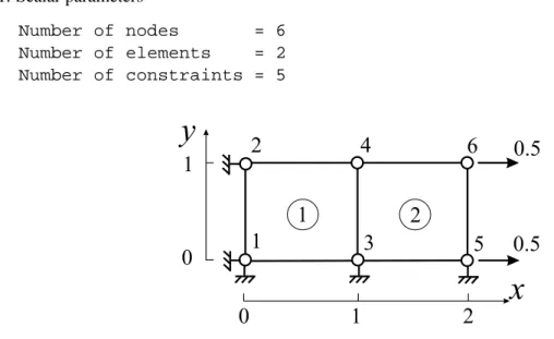
Let us write down numerical information for a simple problem depicted in Fig. 5.1. The finite element model can be described as follows:
1. Scalar parameters
Number of nodes = 6 Number of elements = 2 Number of constraints = 5
1
2
4
6
3
5
y
x
1
0
0
1
2
0.5
0.5
1
2
Figure 5.1: Discrete model composed of two finite elements.
34 CHAPTER 5. DISCRETIZATION
Number of loads = 2
2. Material properties
Elasticity modulus = 2.0e+8 MPa Poisson’s ratio = 0.3
3. Node coordinates (x1,y1,x2,y2etc.)
1) 0 0 2) 0 1 3) 1 0 4) 1 1 5) 2 0 6) 2 1
4. Element connectivity array (counterclockwise direction)
1) 1 3 4 2 2) 3 5 6 4
5. Constraints (node, direction:x= 1;y = 2)
1 1 2 1 1 2 3 2 5 2
6. Nodal forces (node, direction, value)
5 1 0.5 6 1 0.5
While for simple example like the demonstrated above the finite element model can be coded by hand, it is not practical for real-life models. Various automatic mesh generators are used for creating finite element models for complex shapes.
5.2
Mesh generation
5.2.1 Mesh generators
The finite element models for practical analysis can contain tens of thousands or even hundreds of thousands degrees of freedom. It is not possible to create such meshes manually. Mesh generator is a software tool, which divides the solution domain into many subdomains – finite elements. Mesh generators can be of different types.
For two-dimensional problems, we want to mention two types: block mesh generators and trian-gulators.
Block mesh generators require some initial form of gross partitioning. The solution domain is partitioned in some relatively small number of blocks. Each block should have some standard form. The mesh inside block is usually generated by mapping technique.
Triangulators are typically generate irregular mesh inside arbitrary domains. Voronoi polygons and Delaunay triangulation are widely used to generate mesh. Later triangular mesh can be transformed to the mesh consisting of quadrilateral elements. Delaunay triangulation can be generalized for three-dimensional domains.
5.2.2 Mapping technique
Suppose we want to generate quadrilateral mesh inside a domain that has the shape of curvilinear quadrilateral. Mapping technique shown in Fig. 5.2 can be used for this purpose.
If each side of the curvilinear quadrilateral domain can be approximated by parabola then the do-main looks like 8-node isoparametric element. The dodo-main is mapped to a square in the local coordinate
5.2. MESH GENERATION 35
h
h
Dh
Dx
y
x
1
2
3
4
5
6
7
8
9
10
E1
E2
Figure 5.2: Mesh generation with mapping technique.
systemξ, η. The square in coordinatesξ, ηis divided into rectangular elements then nodal coordinates are transformed back to the global coordinate systemx,y.
Algorithm of coordinate calculation for nodei nξ =number of elements inξdirection
nη =number of elements inηdirection Row:R= (i−1)/(nξ+ 1) + 1
Column: C= mod((i−1),(nξ+ 1)) + 1
∆ξ = 2/nξ ∆η = 2/nη ξ=−1 + ∆ξ(C−1)
η=−1 + ∆η(R−1)
x=PNk(ξ, η)xk y=PNk(ξ, η)yk
Connectivities for elemente
Element row: R= (e−1)/nξ+ 1
Element column: C= mod((e−1), nξ) + 1 Connectivities (global node numbers):
i1 = (R−1)(nξ+ 1) +C i2 =i1+ 1
i3 =R(nξ+ 1) +C+ 1
i4 =i3−1
Shifting of midside nodes closer to some corner of the domain helps to refine (make smaller elements) mesh near this corner. If refinement is done on the element side which is parallel to the local axisξand the size of the smallest element near the corner node is∆lthen the midside node should be moved to