Approximate shortest paths in weighted graphs

Contents lists available atSciVerse ScienceDirect

Journal of Computer and System Sciences

www.elsevier.com/locate/jcss

Approximate shortest paths in weighted graphs

Raphael Yuster

Department of Mathematics, University of Haifa, Haifa 31905, Israel

a r t i c l e

i n f o

a b s t r a c t

Article history:

Received 13 October 2010

Received in revised form 5 August 2011 Accepted 6 September 2011

Available online 14 September 2011

Keywords: Shortest path Weighted graph Approximation

We present an approximation algorithm for theall pairs shortest paths(APSP) problem in weighed graphs. Our algorithm solves the APSP problem for weighted directed graphs, with real (positive or negative) weights, up to anadditiveerror of

. For any pair of verticesu,v, the algorithm finds a path whose length is at mostδ(u,v)+

. The algorithm is randomized and runs inO˜(n(ω+3)/2_{) <O(n}2.688_{)time, wherenis the number of vertices and}

_ω

_{is the} matrix multiplication exponent. The absolute weights are allowed to mildly depend upon n, being at mostno(1) _{(we note that even if the weights are constants, δ(u,v) can be}

linear inn, while the error requirement

is a small constant independent ofn). Clearly,

-additive approximations generalize exact algorithms for integer weighted instances. Hence, if

ω

=2+o(1), this algorithm is as fast as any algorithm known for integer APSP in directed graphs, and is more general.

©2011 Elsevier Inc. All rights reserved.

1. Introduction

Shortest paths problems are among the most fundamental algorithmic graph problems. In the shortest paths problem

we are given a (possibly weighted, possibly directed) graph G

=

(

V

,

E

)

and a set S

⊂

V

×

V of pairs of vertices, and are

required to find distances and shortest paths connecting the pairs in S. In theSingle Source Shortest Paths(SSSP) problem we

have S

= {

s

} ×

V for somes

∈

V and in theAll Pairs Shortest Paths(APSP) problem we haveS

=

V

×

V.

Our main result is on the APSP problem. In its most general setting, the graphG

=

(

V

,

E

)

is a directed graph with real

edge weights that can be positive or negative. Thus, the graph is associated with a weight function w

:

E

→

. Algorithms

that manipulate real numbers as pure entities work in the addition-comparison model. In this model the only operations

allowed on pairs of real numbers are additions and comparisons, and each of these operations has unit cost. The fastest

algorithm for the general APSP problem was obtained by Chan [3]. Its runtime forn-vertex graphs is O

(

n3_log3_logn

_/

_log2_n

₎

which is almost cubic. This result improved earlier barely sub-cubic algorithms dating back to the first such algorithm by Fredman [6]. When edge weights are integers, we are no longer restricted to the addition-comparison model, and we can manipulate the bits of the integral weight. The fastest algorithm for APSP in directed graphs with integer (positive or

negative) weights was obtained by Zwick [12] and runs in O

˜

(

n2+μ

)

time,1 where

μ

<

0

.

575 is a function of the exponent

of rectangular matrix multiplication. It is assumed here that the weights are small (their absolute value is bounded by

a constant, or, more liberally, at most no(1)_{). We note that if (as many researcher find plausible) twon}

_×

_{nmatrices can be}

multiplied in O

˜

(

n2

₎

_{time, Zwick’s algorithm, as well as an earlier algorithm of algorithm of Alon, Galil, and Margalit [2],}

runs in O

˜

(

n2.5

₎

_time.

The theoretical and practical importance of the APSP problem lead many researchers to look for faster algorithms that

settle for almost shortest paths. The review article [13] contains a detailed survey of such algorithms. There are two

nat-ural ways to approximate shortest paths. The first is by stretch-factoralgorithms. These types of algorithms guarantee an

E-mail address:[email protected].

1 _{Throughout this paper,O˜}

(f(n))stands for f(n)no(1)_.

0022-0000/$ – see front matter ©2011 Elsevier Inc. All rights reserved.

α

-stretch factor. Namely, they compute a path whose length is at most

α

δ(

u

,

v

)

, where

δ(

u

,

v

)

is the distance fromu tov

(assumed to be positive in this definition), and

α

>

1. The second isadditive approximations (also calledsurplus

approxi-mations). These types of algorithms guarantee an

-additive error. Namely, they compute a path whose length is at most

δ(

u

,

v

)

+

. The fastest stretch-factor algorithm for APSP was obtained by Zwick [12]. His algorithm achieves a stretch of

(

1

+

)

inO

˜

((

nω

/

)

log

(

W

/

))

time. The algorithm assumes that the real weights are all positive and in the interval

[

1

,

W

]

.

If

=

1

/

nt_{, andt}

₀

_.

_{706, and W}

₌

_no(1)_{, then a faster algorithm whose runtime is O}

˜

₍

_nω+0.468t

₎

_{was obtained by Roditty}

and Shapira [10]. Here and throughout this paper

ω

<

2

.

376 denotes the matrix multiplication exponent [4].

Good additive approximations exist forundirected graphs. We mention two notable results. Aingworth, Chekuri, Indyk,

and Motwani [1] obtained a 2-additive APSP algorithm in unweighted undirected graphs that runs in O

˜

(

n2.5

₎

_{time. This was}

later improved by Dor, Halperin, and Zwick [5] who obtained a running time ofO

˜

(

min

{

n3/2_m1/2

_,

_n7/3

_}

₎

_{. They also obtain an}

O

(

logn

)

-additive APSP algorithm that runs in almost optimal O

˜

(

n2

)

time.

It is much more difficult to obtain good additive approximations for directed graphs, moreover for the general case where the weights are real, and possibly negative. One naive approach is to round (up) the real weights to the closest rational

which is a multiple of some O

(

1

/

n

)

. This reduces the problem to computing exact solutions in integer weighted directed

graphs where the absolute weights are O

(

n

)

. However, there is no truly sub-cubic algorithm known that handles such

large integer weights. Likewise, one can obtain a constant additive approximation using the stretch factor approximation

algorithm of Zwick mentioned above, with

=

O

(

1

/

n

)

. However, this also results in a super-cubic runtime, and, in addition,

does not directly apply to the case of negative edge weights.

Our main result obtains the first truly sub-cubic algorithm that achieves an

-additive approximation. It applies to the

most general setting, where positive and negative real weights are allowed. It is assumed that the absolute value of a weight

is at mostno(1).

Theorem 1.1.Let

>

0be fixed. Let G

=

(

V

,

E

)

be a directed graph whose edges have real(positive or negative)weights, of absolute value at most no(1)_{. There is a randomized algorithm that computes APSP in G up to an}

_{-additive error in}

_O

˜

₍

_n(ω+3)/2

₎

_time.

We assume that the input graph contains no negative cycles. In other words, for pairsu

,

v for which

δ(

u

,

v

)

= −∞

, the

result returned by the algorithm is meaningless. Clearly, any

-additive approximation algorithm implies an exact algorithm

for the case of integer weights. The converse, however, is not necessarily true. Hence, the algorithm of Theorem 1.1 is also

an O

˜

(

n(ω+3)/2

₎

_{exact algorithm for the case of small (positive or negative) integer weights. This matches the runtime of the}

algorithm of Alon, Galil, and Margalit [2], but is strictly more general than it. In fact, if

ω

=

2

+

o

(

1

)

, then the runtime of the

algorithm of Theorem 1.1 matches the runtime of the fastest known integer APSP algorithm of Zwick mentioned earlier. The

algorithm of Theorem 1.1, though, is strictly more general as it can handle real weights, while still obtaining an

-additive

error.

The rest of this paper contains the proof of Theorem 1.1 in Section 2 and some concluding remarks and open problems in Section 3.

2. Proof of the main result

We construct a weight-approximated version of the input graph that is somewhat easier to work with. Let Gint be

obtained fromG be replacing each weight w

(

e

)

with the weight wint

(

e

)

=

2nw

(

e

)

. Since 0

wint

(

e

)

−

2nw

(

e

) <

1 we

know that whenever

δ(

u

,

v

)

is finite, then

δ

int

(

u

,

v

)

is also finite and 0

δ

int

(

u

,

v

)

−

2n

δ(

u

,

v

) <

n. Hence, in order to obtain

-additive approximations of distances in G it suffices to obtainn-additive approximations

δ

ˆ

int of distances in Gint, since

such an approximation implies

δ(

u

,

v

)

2n

δ

ˆ

int

(

u

,

v

)

δ(

u

,

v

)

+

.

It is our goal, therefore, to compute an approximation

δ

ˆ

int

(

u

,

v

)

of lengths of actual paths inGint that satisfies

δ

int

(

u

,

v

)

δ

ˆ

int

(

u

,

v

)

δ

int

(

u

,

v

)

+

n

.

Denote byW the maximum absolute value of a weight of an edge ofG, and recall thatW

=

no(1)_{. For any two vertices}

u

,

v we have

|

δ(

u

,

v

)

|

<

nW (from here onwards we will only consider pairs for which

δ(

u

,

v

)

, and thus

δ

int

(

u

,

v

)

, is finite).

Each weight ofGint is an integer in

{−

K

, . . . ,

K

}

whereK

=

(

2W

/

)

n

+

1

. Notice, though, that distances inGintcan be of

absolute value as large as O

˜

(

n2

)

.

2.1. Computing distances for a given subset of pairs

An important part of our algorithm consists of computing exact distances in Gint for all pairs in a set of pairs

S

×

V

∪

V

×

S, where S is relatively large, but still a small part of V. In other words, we will solve SSSP in Gint from

each vertex of S, and solve SSSP in theedge-reversed Gint from each vertex of S. It is costly, though, to compute SSSP in

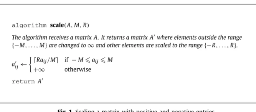
algorithm scale(A,M,R)

The algorithm receives a matrix A. It returns a matrix Awhere elements outside the range {−M, . . . ,M}are changed to∞and other elements are scaled to the range{−R, . . . ,R}. a_{i j}←

Rai j/M if −Mai jM

+∞ otherwise

returnA

Fig. 1.Scaling a matrix with positive and negative entries.

for justoneapplication of SSSP and then reduce the problem to SSSP in a graph with non-negative edge weights. Johnson’s

reweighing consists of running a single application of SSSP from a new vertex, denoted byr, connected with directed edges

of weight 0 fromrto each vertex ofV. Goldberg [7], improving a result of Gabow and Tarjan [8], obtained an O

(

m

√

nlogK

)

algorithm for the SSSP problem in directed graphs with integer edge weights of value at least

−

K (herem

=

O

(

n2

₎

_denotes

the number of edges of the graph). It follows that the reweighing of Gint can be obtained in O

˜

(

n2.5

)

time, in our case. The

reweighing consists of assigning vertex weightsh

(

v

)

for eachv

∈

V (these are the distances fromrto vafter applying SSSP

fromr). The new weight, denoted bywint+

(

u

,

v

)

is justwint

(

u

,

v

)

+

h

(

u

)

−

h

(

v

)

0. It now suffices to compute S S S Pfrom

each vertex of SinGint+(and similarly in its edge-reversed version). This, in turn, can be performed inO

(

n2

)

time for each

vertex of S, using Dijkstra’s algorithm. We therefore obtain:

Lemma 2.1.Let S

⊂

V . There is an algorithm that computes

δ

int

(

s

,

v

)

and

δ

int

(

v

,

s

)

for each s

∈

S and each v

∈

V inO

˜

(

|

S

|

n2

+

n2.5

)

time.

Recall that Dijkstra’s algorithm also computes shortest paths trees, hence a representation of shortest paths yielding the distances can be efficiently computed in the same time.

2.2. Approximating distances that are realized by few edges

Another important part of our algorithm consists of computingapproximatedistances inGintconnecting pairs of vertices

for which there exists a shortest path (realizing the exactdistance) that does not use too many edges. More precisely, for

a pair of verticesu

,

v, letc

(

u

,

v

)

be the smallest integerksuch that

δ

int

(

u

,

v

)

is realized by a path containingkedges. We

describe a procedure that obtains ann-additive approximation of

δ

int

(

u

,

v

)

for those pairsu

,

v havingc

(

u

,

v

)

t, wheret

will be chosen later. Notice that ifc

(

u

,

v

)

t, then

|

δ

int

(

u

,

v

)

|

K t.

Our procedure is a modified version of the stretch-factor approximation algorithm of Zwick from [12], although the latter only applies to graphs with positive edge weights. Indeed, let us first show how Zwick’s algorithm can be applied, without

change, in the special case where G (and hence Gint) only has positive edge weights. In this case, each edge of Gint is in

{

1

, . . . ,

K

}

. For a given

γ

>

0, the algorithm from [12] computes paths of stretch at most 1

+

γ

in time O

˜

((

nω

/

γ

)

logK

)

.

If we apply it with

γ

=

/(

2W t

)

the running time becomes, in our case,O

˜

(

tnω

)

. It computes paths of length

δ

ˆ

int

(

u

,

v

)

, of

stretch at most 1

+

γ

, for all pairs of vertices of Gint. But let us examine what this means for those pairs havingc

(

u

,

v

)

t.

For such pairs we have

ˆ

δ

int

(

u

,

v

)

(

1

+

γ

)δ

int

(

u

,

v

)

=

δ

int

(

u

,

v

)

+

2W t

δ

int

(

u

,

v

)

δ

int

(

u

,

v

)

+

2W tK t

δ

int

(

u

,

v

)

+

n

.

The stretch-factor approximation is meaningless when negative weight edges (and hence paths) exist. Still, we can modify

the algorithm from [12] so that its consequence for additive approximations of those pairs for which c

(

u

,

v

)

t remains

almost intact. The modification will still run in O

˜

(

tnω

)

time, but its analysis will be somewhat more involved.

Recall that a weighted directed graph, such asGint, is associated with itsdistance matrix. This matrix, denoted byD, has

rows and columns indexed by V and has D

(

u

,

v

)

=

wint

(

u

,

v

)

. We assume that diagonal entries are 0 and if there is no

edge from u to v then D

(

u

,

v

)

= ∞

. If D1 and D2 are two distance matrices then the matrix C

=

D1

D2 is defined by

C

(

u

,

v

)

=

minw∈VD1

(

u

,

w

)

+

D2

(

w

,

v

)

. We callC thedistance productofD1andD2. We also denoteD2

=

D

D (not to be

confused with the standard matrix product). Notice that D2

₍

_u

_,

_v

₎

_{is theexactdistance fromu to v wheneverc}

₍

_u

_,

_v

₎

_2.

Similarly Di

=

Di−1

D (and which, by associativity, equals also Dj

Di−j for any j

=

1

, . . . ,

i

−

1) has the property that

Di

(

u

,

v

)

is the exact distance fromuto vwheneverc

(

u

,

v

)

i.

It is therefore our goal to approximate the entries of Dt

₍

_u

_,

_v

₎

_{. We will show how to compute a matrix Bso that for any}

pair u

,

v we have Dt

(

u

,

v

)

B

(

u

,

v

)

Dt

(

u

,

v

)

+

n, thereby obtaining ann-additive approximation for those pairs having

c

(

u

,

v

)

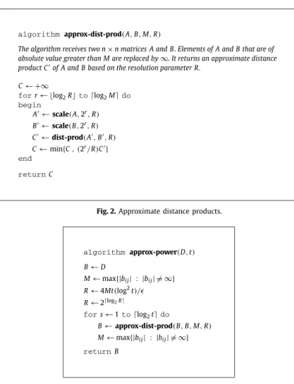
t.

The procedure is based on exact distance products of scaled versions of the matrices to be (distance) multiplied. The

algorithm approx-dist-prod(A,B,M,R)

The algorithm receives two n×n matrices A and B. Elements of A and B that are of absolute value greater than M are replaced by∞. It returns an approximate distance product Cof A and B based on the resolution parameter R.

C← +∞

forr← log2Rtolog2Mdo begin A←scale(A,2r ,R) B←scale(B,2r_,R) C←dist-prod(A,B,R) C←min{C, (2r_/R)C} end returnC

Fig. 2.Approximate distance products.

algorithm approx-power(D,t) B←D M←max{|bi j| : |bi j| = ∞} R←4Mt(log2t)/ R←2log2R fors←1tolog2tdo B←approx-dist-prod(B,B,M,R) M←max{|bi j| : |bi j| = ∞} returnB

Fig. 3.Computing an approximation ofDt_.

that it also scales matrices with negative entries. The elements of a matrix A in the range

{−

M

, . . . ,

M

}

are scaled (and

rounded up) to the range

{−

R

, . . . ,

R

}

. Other elements are replaced with infinity. Algorithm scale is used by algorithm

approx-dist-prod

(

A

,

B

,

M

,

R

)

, given in Fig. 2, whose code is identical to the one from [12] (but we will apply it on matrices

that also have negative entires). Algorithmapprox-dist-prodcomputes an approximation of the distance product A

B.

Suppose Ris a power of 2 and that every finite element in A andB is in

{−

M

, . . . ,

M

}

. LetC

=

A

B and letC be the

matrix obtained by callingapprox-dist-prod

(

A

,

B

,

M

,

R

)

. The same analysis as in [12] shows that for everyi and j,

c_{i j}

ci j

ci j

+

2M

/

R

.

(1)

We show how to compute an approximation of Dt _{by repeated applications ofapprox-dist-prod. We will assume thatt}

is a power of 2, and compute the approximation by repeated squaring, as shown in Fig. 3.

Let us setRto be the smallest power of 2 greater than 4W t

(

log2t

)/

. LetMsbe the value ofMthat is set during thes’th

iteration in algorithmapprox-power. Likewise, letBsbe the matrix Bduring thes’th iteration in algorithmapprox-power.

The following lemma establishes bounds onMs and on the entries of Bs.

Lemma 2.2.In round s of algorithmapprox-powerwe have:

Ms

2sK

_s

j=0

s j

Rj

,

D2s

(

i

,

j

)

Bs

(

i

,

j

)

D2 s

(

i

,

j

)

+

2sK

_s

j=1

s j

Rj

.

Proof. The proof is by induction ons. Fors

=

1, note that in the first call toapprox-dist-prod, each finite element ofB

=

D

has a value in

{−

K

, . . . ,

K

}

, and K

=

M. Thus, by Eq. (1), in the resulting B1 we haveD2

(

i

,

j

)

B1

(

i

,

j

)

D2

(

i

,

j

)

+

2K

/

R.

assume that the lemma holds for s

−

1 and prove it for s. In the call to approx-dist-prodduring iteration s, each finite

element of B

=

Bs−1has a value in

{−

Ms−1

, . . . ,

Ms−1

}

, andM

=

Ms−1. Thus, in resulting Bswe have

B2_s−1

(

i

,

j

)

Bs

(

i

,

j

)

B2s−1

(

i

,

j

)

+

2Ms−1

/

R

.

On the other hand, by the induction hypothesis, D2s−1

(

i

,

j

)

Bs−1

(

i

,

j

)

D2 s−1

(

i

,

j

)

+

2s−1K

_s−1

j=1

_s−1 j

Rj

,

from which it follows that

D2s

(

i

,

j

)

B2_s−1

(

i

,

j

)

D2s

(

i

,

j

)

+

2sK

_s−1

j=1

s−1 j

Rj

.

Therefore, D2s

(

i

,

j

)

Bs

(

i

,

j

)

D2 s

(

i

,

j

)

+

2sK

_s−1

j=1

s−1 j

Rj

+

2Ms−1

/

R

D2s

(

i

,

j

)

+

2sK

_s−1

j=1

s−1 j

Rj

+

2 R2 s−1_K

_s−1

j=0

s−1 j

Rj

=

D2s

(

i

,

j

)

+

2sK

_s

j=1

s j

Rj

.

Similarly, Ms

2Ms−1

+

2Ms−1

/

R

=

2Ms−1

(

1

+

1

/

R

)

2sK

_s−1

j=0

_s−1 j

Rj

(

1

+

1

/

R

)

=

2sK

_s

j=0

_s j

Rj

.

2

Lemma 2.3.The matrix B computed byapprox-powersatisfies Dt

₍

_u

_,

_v

₎

_B

₍

_u

_,

_v

₎

_Dt

₍

_u

_,

_v

₎

₊

_{n for all pairs u}

_,

_{v. The running} time ofapprox-powerisO

˜

(

nωt

)

.

Proof. By our choice ofR as the smallest power of 2 greater than 4W t

(

log2t

)/

we have, from Lemma 2.2, that fors

=

logt,

Dt

(

u

,

v

)

B

(

u

,

v

)

Dt

(

u

,

v

)

+

t K

_s

j=1

_s j

Rj

<

Dt

(

u

,

v

)

+

t Klog2t

/

R

<

Dt

(

u

,

v

)

+

K

/(

4W

) <

Dt

(

u

,

v

)

+

n

.

The running time follows from the fact that we apply a polylogarithmic number of calls to dist-prod, which, in turn, runs

in O

˜

(

Rnω

)

= ˜

O

(

nωt

)

, as shown by Yuval [11] (see also [12]).

2.3. Completing the proof of Theorem 1.1

We sett to be the smallest power of two larger thann(3−ω)/2_.

We first apply the algorithm of Lemma 2.3 which computes a value B

(

u

,

v

)

for each pair of verticesu

,

v. By Lemma 2.3,

this requires O

˜

(

n(ω+3)/2

₎

_{time. Next, we choose a random subset S}

_⊂

_{V consisting of 4nlnn}

_/

_{t vertices. We apply the}

algorithm of Lemma 2.1 and obtain

δ

int

(

s

,

v

)

and

δ

int

(

v

,

s

)

for each s

∈

S and each v

∈

V. By Lemma 2.1, this requires

˜

O

(

n(ω+3)/2

₎

_{time. For each pair of verticesu}

_,

_{v let}

(

u

,

v

)

=

min

s∈S

δ

int

(

u

,

s

)

+

δ

int

(

s

,

v

).

Notice that the runtime required for computing all the

(

u

,

v

)

is also O

˜

(

n(ω+3)/2

₎

_.

Our algorithm will return, for each pairu

,

v, the value

ˆ

δ

int

(

u

,

v

)

=

min

B

(

u

,

v

), (

u

,

v

)

.

We claim that with very high probability,

δ

int

(

u

,

v

)

δ

ˆ

int

(

u

,

v

)

δ

int

(

u

,

v

)

+

n. Consider a pair of vertices u

,

v for which

c

(

u

,

v

) >

t. Let p

(

u

,

v

)

be some path with c

(

u

,

v

)

edges, realizing

δ

int

(

u

,

v

)

. As S was chosen randomly, the

probabil-ity that none of the (at least t) internal vertex of p

(

u

,

v

)

belongs to S is at most

(

1

−

(

4 lnn

)/

t

)

t

<

1

/

n3. Hence, with

probability at least 1

−

1

/

n, S has the property that for each pair u

,

v withc

(

u

,

v

) >

t, there is some path with c

(

u

,

v

)

that sub-paths of shortest paths are shortest paths, that

(

u

,

v

)

=

δ

int

(

u

,

v

)

wheneverc

(

u

,

v

) >

t. On the other hand, for

pairs u

,

v withc

(

u

,

v

)

t, we have, by Lemma 2.3, that Dt

₍

_u

_,

_v

₎

_B

₍

_u

_,

_v

₎

_Dt

₍

_u

_,

_v

₎

₊

_{n. But sincec}

₍

_u

_,

_v

₎

_{t, we have}

Dt

(

u

,

v

)

=

δ

int

(

u

,

v

)

, and hence

δ

int

(

u

,

v

)

B

(

u

,

v

)

δ

int

(

u

,

v

)

+

n.

We have proved that, with probability at least 1

−

1

/

n, for all pairs u

,

v for which

δ

int

(

u

,

v

)

is finite, we have

δ

int

(

u

,

v

)

δ

ˆ

int

(

u

,

v

)

δ

int

(

u

,

v

)

+

n. Also notice that our approximation

δ

ˆ

int

(

u

,

v

)

represents an actual path having this

length. A data structure representing the actual paths is also easily obtained. For

(

u

,

v

)

this is obtained by the shortest

path trees constructed by Dijkstra’s algorithm (as noted in the paragraph following Lemma 2.1). For B

(

u

,

v

)

this is obtained

using the witnesses ofdist-prod, as shown in [12].

2

3. Concluding remarks

The algorithm of Theorem 1.1, running in O

˜

(

n(ω+3)/2

₎

_{, is asymptotically as fast as any known algorithm for integer}

APSP, if

ω

=

2

+

o

(

1

)

. Still, for the current known upper bound of

ω

, Zwick’s algorithm for integer APSP runs faster, in

˜

O

(

n2+1/(4−ω)

₎

_{time (and even slightly faster using rectangular matrix multiplication). Although it is of some interest to}

improve the runtime of the algorithm of Theorem 1.1 to match the runtime of Zwick’s algorithm, the major task is, clearly,

to break theO

˜

(

n2.5

₎

_{barrier assuming}

_ω

₌

₂

₊

_o

₍

₁

₎

_.

References

[1] D. Aingworth, C. Chekuri, P. Indyk, R. Motwani, Fast estimation of diameter and shortest paths (without matrix multiplication), SIAM J. Comput. 28 (1999) 1167–1181.

[2] N. Alon, Z. Galil, O. Margalit, On the exponent of the all pairs shortest path problem, J. Comput. System Sci. 54 (1997) 255–262.

[3] T.M. Chan, More algorithms for all-pairs shortest paths in weighted graphs, in: Proceedings of the 39th ACM Symposium on Theory of Computing (STOC), ACM Press, 2007, pp. 590–598.

[4] D. Coppersmith, S. Winograd, Matrix multiplication via arithmetic progressions, J. Symbolic Comput. 9 (1990) 251–280. [5] D. Dor, S. Halperin, U. Zwick, All pairs almost shortest paths, SIAM J. Comput. 29 (2000) 1740–1759.

[6] M.L. Fredman, New bounds on the complexity of the shortest path problem, SIAM J. Comput. 5 (1976) 49–60. [7] A.V. Goldberg, Scaling algorithms for the shortest paths problem, SIAM J. Comput. 24 (1995) 494–504.

[8] H.N. Gabow, R.E. Tarjan, Faster scaling algorithms for general graph matching problems, J. ACM 38 (1991) 815–853. [9] D.B. Johnson, Efficient algorithms for shortest paths in sparse graphs, J. ACM 24 (1977) 1–13.

[10] L. Roditty, A. Shapira, All-Pairs Shortest Paths with a sublinear additive error, in: Proceedings of the 35th International Colloquium on Automata, Languages, and Programming (ICALP), in: Lecture Notes in Comput. Sci., 2008, pp. 622–633.

[11] G. Yuval, An algorithm for finding all shortest paths usingN2.81_{infinite-precision multiplications, Inform. Process. Lett. 4 (1976) 155–156.}

[12] U. Zwick, All-pairs shortest paths using bridging sets and rectangular matrix multiplication, J. ACM 49 (2002) 289–317.

[13] U. Zwick, Exact and approximate distances in graphs – A survey, in: Proceedings of the 9th Annual European Symposium on Algorithms (ESA), in: Lecture Notes in Comput. Sci., 2001, pp. 33–48.