GPU ACCELERATED HUNGARIAN ALGORITHM FOR TRAVELING SALESMAN PROBLEM
BY
VARSHA RAVI PRAKASH KAUSHIK
THESIS
Submitted in partial fulfillment of the requirements for the degree of Master of Science in Industrial Engineering
in the Graduate College of the
University of Illinois at Urbana-Champaign, 2017
Urbana, Illinois
Adviser:
Abstract
In this thesis, we present a model of the Traveling Salesman Problem (TSP) cast in a quadratic assignment problem framework with linearized objective function and constraints. This is referred to as Reformulation Linearization Technique at Level 2 (or RLT2). We apply dual ascent proce-dure for obtaining lower bounds that employs Linear Assignment Problem (LAP) solver recently developed by Date [1]. The solver is a parallelized Hungarian Algorithm that uses Compute Unified Device Architecture (CUDA) enabled NVIDIA Graphics Processing Units (GPU) as the parallel programming architecture. The aim of this thesis is to make use of a modified version of the Dual Ascent-LAP solver to solve the TSP.
Though this procedure is computational expensive, the bounds obtained are tight and our ex-perimental results confirm that the gap is within 2% for most problems. However, due to limitations in computational resources, we could only test problem sizesN <30. Further work can be directed at theoretical and computational analysis to test the efficiency of our approach for larger problem instances.
Acknowledgments
I would like to thank my adviser, Professor Rakesh Nagi, for his immense support and guidance towards this thesis. I am grateful to him for being extremely patient with me, encouraging me and helping me at every step.
I would like to express my sincere gratitude towards Ketan Date, for helping me more than I could’ve asked for!
Finally, a big thank you to my family and to all my friends at Urbana - Champaign and back in India who have been constants in lifting up my spirits every time I needed them. Kartik, Tooba, Banu, Supraja and Subha - thank you so much for making this journey easy for me.
Contents
List of Tables . . . vi
List of Figures . . . vii
Chapter 1 Introduction . . . 1
1.1 Traveling Salesman Problem and its Variants . . . 1
1.2 Organization of the Thesis . . . 3
Chapter 2 Literature Review . . . 4
Chapter 3 Reformulation Linearization Technique for the TSP in a QAP framework . . . 11
3.1 Quadratic Assignment Problem (QAP) . . . 11
3.2 Reformulation Linearization Technique . . . 13
3.3 QAP representation of the TSP . . . 15
Chapter 4 Solution Approach . . . 20
4.1 Dual Ascent . . . 20
4.2 Hungarian Algorithm . . . 22
4.3 Accelerating RLT2-DA Algorithm for the TSP Using a GPU Cluster . . . 24
4.4 Computational Experiments . . . 25
Chapter 5 Conclusions . . . 27
List of Tables
3.1 Percentage reduction in the number of variables from QAP to TSP . . . 18
3.2 Comparison of Integer vs Linear Programming formulation . . . 19
4.1 Comparison of Solution times of QAP and reformulated TSP . . . 25
4.2 Solution times for instances from TSPLIB TSP . . . 26
List of Figures
Chapter 1
Introduction
1.1
Traveling Salesman Problem and its Variants
Traveling Salesman Problem (TSP) is one of the most popular problems studied under the combinatorial optimization problem set. Owing to its NP-hard (non-deterministic polynomial-time hard) nature, the problem is challenging to solve optimally. Despite progress, there remains a need for efficient solution methods due to its wide applicability in various practical fields. TSP can be defined as the problem of finding the minimum cost tour among a given pair of cities such that a salesman visits every city exactly once with the cost metric defined in terms of distance, time, etc. One of the most common integer programming formulations for the TSP can be written as:
Objective: minX i X j6=i Cijxij (1.1) s.t. X i xij = 1 ∀j (1.2) X j6=i xij = 1 ∀i (1.3) ui−uj+nxij ≤n−1, 2≤i6=j≤n (1.4) xij ∈ {0,1} ∀i, j (1.5)
xij = 1 if salesman travels directly from locationitoj; 0 otherwise
dij the distance between citiesiand j
Objective= min total distance traveled in a tour (1.2) ensures salesman arrives once at each city (1.3) ensures salesman leaves each city once
(1.4) enforces there is a single tour covering all cities
The applications of the TSP encompass a comprehensive list with the most common ones being vehicle routing problem and its variations (see Laporte, 1992), tool head path planning for drilling VSLI circuit boards, computer wiring (Lenstra and Rinnooy Kan, 1975), hole punching (Reinelt, 1989), several manufacturing contexts, job sequencing, dartboard design (Eiselt and La-porte, 1991), crystallography (Bland and Shallcross, 1989), crew scheduling, etc. Variants to the TSP are used to represent particular situations and to model them accurately. Broadly, routing problems can be divided into static and dynamic problems. When all required input data of the problem are known before routes are calculated, it is considered a static routing problem. If, on the other hand, some of the input data are obtained during the execution of a route, it is a dynamic problem. In this section, we describe a few variants (see also, Fig. 1).
Asymmetric TSP (ATSP): A variant of the TSP, based on the connections between each node, is classified into symmetric or asymmetric types. A symmetric TSP is one in which the cost function between two nodes will be the same regardless of the direction of travel, while in an asymmetric TSP cost functions between nodes are dependent on the direction of travel.
TSP with Multiple Visits (TSPM): TSP is generally formulated as Euclidean TSP where distance matrix D is expected to be symmetric dij =dji for all i, j, and to satisfy triangle
inequality dik ≤dij+djk for all distincti, j, k. A TSP, without triangle inequality becomes a TSP
with multiple visits (TSPM) where the constraint of having to visit each node exactly once may be relaxed [2]. In general, the TSPM can be defined as the problem of findingm minimum cost tours form (more than one) salesmen, starting and ending at a depot/node, such that each intermediate node is visited exactly once.
TSP with Multiple Salesmen (mTSP): In the multiple TSP (mTSP), m identical salesmen are used to visit each customer exactly once, each salesman starting from a single depot and returning to the same location. The objective of the mTSP is mostly to minimize the total distance traveled by m salesmen, with a bound on the number of salesmen. In literature, mTSPs are mostly utilized to solve VRPs.
Max TSP: The objective of the max TSP is to find a tour with the maximum cost, unlike other TSPs. The condition for a salesman is that every city is visited exactly once with the same starting and return location. The problem can be solved as a conventional TSP by replacing each edge in the tour by its additive inverse.
Generalized TSP (GTSP): An extension of the TSP is a Generalized Traveling Sales-man Problem (GTSP) in which nodes of the graph are grouped into clusters and the expected solution is a minimum cost tour in which either exactly one city from each cluster is visited or in
which at least one city from each cluster is visited.
Clustered TSP: In a clustered TSP, the nodes of the graph are grouped into clusters and the solution is a tour with minimum cost subject to the condition that cities from a cluster are visited consecutively. This problem can be converted to a simple TSP by treating each cluster as a node by adding a largeM to each inter-cluster edge.
TSP with Time Windows (TSPTW): In the TSP with time windows (TSPTW), job at customerimust be completed within the time interval{ai,bi}whereai is the earliest allowable
service start time for customer i. If the salesman arrives prior to time ai, the salesman will wait
without penalty. The time required for service is given bysi and its value lies within 0 andbi−ai.
The problem in the TSPTW is to find a tour with minimum cost, each customer visited exactly once within their accepted time windows.
Time dependent TSP: In time dependent TSP, the cost of traveling from a city ito city j, defined as ctij wheret={1,2, ..., n}, is dependent on the time of travel t. The objective is to find a tour starting and ending at the same city with each city visited exactly once, such that the sum of cost of traveling from cityito city j ∀i, j,
n
P
i=1
cti(i+1) is minimized.
Reward seeking TSP: In this class of the TSP variant, every customer is associated with a value. The constraint of having to visit every customer at least once can be relaxed since it might be beneficial to visit a customer with higher value at the cost of some other customer. However, any given customer can only be visited at most once. Within this class, there are multiple variants: Prize collecting TSP (PTSP), Profitable Tour Problem (PTP), Orienteering and Team Orienteering Problem (OP & TOP), TSP with profits (TSPP).
A brief literature review has been provided for these variants in the following chapter.
1.2
Organization of the Thesis
The next chapter provides a brief literature review of the TSP and its variants. Chapter 3 discusses the QAP, Reformulation Linearization Techniques and compares the results obtained RLT1 and RLT2 for a set of problem instances. Chapter 4 discusses the solution approach for the TSP in a QAP framework. It discusses the parallelization of the alternating tree variant of the Hungarian Algorithm and the Lagrangian Dual Ascent approach for calculating strong lower bounds on RLT2 for QAP and TSP.
Chapter 2
Literature Review
The computational times for solving a TSP is of the order proportional to O(n!), n being the number of cities/nodes in the system. With the increase in the number of nodes, solution space increases exponentially, since the TSP an NP-hard problem. TSP was first coined in 1930, and ever since, a plethora of exact and heuristic solution methods have been suggested to solve the TSP and ATSP. Initial notable contributions were made by Dantzig, Fulkerson and Johnson [3] during the 1950s. The authors used undirected graphs and expressed a problem of finding the shortest path for a Hamiltonian cycle of 49 cities as an integer linear program with inequality restraints (cuts, shown below) that could be added gradually to the formulation using a branch and bound scheme to eliminate sub tours and reach the optimal solution.
X
i,j∈S
Xij ≤ |S| −1, S⊆ {2, ..., n},2≤ |S| ≤n−1 (2.1)
Morton and Land [4] suggested a linear programming formulation for the TSP with the objec-tive of finding the shortest tour for a set of nodes such that there are no sub-tours. Since an LP representation has sub-tour formations, the authors used dynamic programming instead of enumer-ating all possible circuits. The procedure involved representing the set of distances between two points as a square matrix and selecting a set of n links to form an initial single loop circuit. The circuit is then changed by simultaneously removing and introducing three new links such that the single loop is always maintained.
Barachet [5] in his paper used the graphical method to describe an enumeration scheme for computing near-optimal tours. The method involved drawing a closed circuit that passed through all N points in the problem. Next step was to form N groups of three consecutive sections to make up a route of minimum length for the section. This process was iteratively performed till a minimum length route was formed. The same operation was repeated for everyN group of 4, 5, 6,
up to (N −1) consecutive sections and then for the unique group of N consecutive sections. This method was shown to be simpler and faster than the one where all possible circuits are considered. Balinski and Gomory [6] in their work, presented a primal method for the assignment and transportation problems. This method, a dual to the Hungarian, provides an orthogonal dual feasible vector (U, V) to the primal infeasible vector X at each intermediate computational step. The method described provides a feasible X (a complete assignment or transportation solution) and a corresponding orthogonal (U, V) at each step providing a constantly improving solution. In [7], Bellman has shown the use of TSP as an example of a combinatorial problem and solved using dynamic programming.
Little et al. [8] coined the term Branch and Bound and presented this algorithm for solving a traveling salesman problem. In this algorithm, a set of feasible solutions is broken up into subsets using the method of branching based on the presence of an edge in the tour. Each branch is solved to obtain a lower bound on the solution. The process is repeated till a subset containing a single tour with length less than or equal to some lower bound for every tour is found. Though the time taken to solve the problem using the branch and bound method increases exponentially with increase in the problem size, this method proved to be faster than most other known methods. Miliotis [9] introduced the cutting plane algorithm which used Gomory cuts to solve the traveling salesman problem.
Miller et al. [10] proposed the earliest known formulation of the ATSP. They used a variable ui to define the order in which a city/node was visited in a tour and the number of vertices in each
route was limited. The sub-tour elimination constraints of the MTZ formulation was given as ui−uj+ (n−1)xij ≤n−2, i, j ={2, ...., n} (2.2)
1≤ui ≤n−1, i={2, ...n} (2.3)
Sherali and Driscoll [11] first applied the Reformulation Linearization Technique (RLT) for the Asymmetric Traveling Salesman Problem (ATSP) formulation for obtaining tighter bounds. This formulation was based on the Miller-Tucker-Zemlin (MTZ) sub-tour elimination constraints. The procedure involved applying a partial first level version of the RLT to a nonlinear MTZ sub-tour elimination constraints, with a variableyij representing the arc (i, j) on the tour,yij 6= 0. Wong [12]
formulated the ATSP as a Multi-Commodity Flow model using non-negative variables to describe the flow of commodities between vertices. The flow variable wijpq was assigned the value 1 if and only if the commodity going fromp toq also flowed on arc (i, j).
Diaby [13] proposed a network-flow based linear programming formulation of the TSP as a relaxation to an Integer programming formulation. A non-linear TSP was remodeled to achieve an Integer Linear program with a framework of graphG= (V, A) where nodes inV correspond to city
and travel stage pairs and the arcs representing travel between two cities at stagesiand i+ 1. The approach developed a reformulation of a standard assignment polytope with variables represented as functions of the flow associated and arcs of the graph.
In the paper [14], Quadratic Traveling Salesman Problem (QTSP) is presented with a quadratic objective aimed at finding a minimum cost tour, where costs are associated to each triple of nodes traveled in series. The authors present three exact algorithms to solve the QTSP: by transforming a QTSP to a Symmetric TSP, by using the branch-and-bound and branch-and-cut algorithms. They also present several simple heuristics, such as Cheapest-Insert Heuristic (CI), a generalization of an ATSP heuristic where they start with an arc (v1, v2) ∈A considered as a cycle such that the cost of a cycle x−v1−v2−x is minimal and new nodes are included iteratively to the cycle in a greedy manner keeping the new cycle cost minimal in each step. The paper also describes other adaptations of generalization of heuristics, Nearest-Neighbor Heuristic, Two-Directional-Nearest-Neighbor Heuristic, Assignment-Patching Heuristic and Nearest-Two-Directional-Nearest-Neighbor-Patching Heuristic, to name a few.
In [15], a lower bounding procedure for the AQTSP has been discussed. First, the AQTSP is transformed to an MILP formulation using two basic steps - reformulation and linearization and then solved via Column Generation (CG) with each cycle represented by a variable. The number of variables is exponentially large and hence constraints were added to the objective and the resulting Lagrangian dual was solved using a dual-ascent strategy. Optimal Lagrangian multipliers were obtained using a subgradient optimization technique. A stabilized column generation method was used to counter the slow convergence and tailing off effects of the regular column generation method. Lower bounds were calculated by solving the pricing problem with the master problem giving a lower bound for the original problem when no more columns can be priced out.
Diaby, Karwan and Sun [16] presented a polynomial-sized linear program (LP) using flow perspective for a TSP over an Assignment Problem - based graph with nodes representing (city, time-of-travel) pairs, and arcs representing travel legs. The novel feature in their model was having variables representing doublets and triplets of travel legs, thus building enough information into the variables in the model and the constraints were enforced by implicitly setting appropriate variables to zero. This led to anO(n9) variables,O(n8) constraints model.
Flood [17] showed the similarities between a traveling salesman problem and an assignment problem and presented a method to solve the assignment problem. He also showed techniques that could be used to obtain good approximate solutions for the symmetric TSP and modifications to the traveling-salesman problem for easier subsequent computations. Kuhn [18] introduced the Hungarian Method for solving the Assignment Problem. Flood described a heuristic approach to solve the TSP using the conditions and notations presented by Kuhn. In this approach, each of the assignment combinations is assigned a numerical rating and the optimal assignment combination is the one that has the least sum of applicable ratings.
To an extent, heuristics have proven to be successful in finding solutions for the basic TSP. However, TSP variants impose significant challenges and heuristic methodologies haven’t been successful.
Multiple TSP
Mole et al. [19] provide several algorithms and heuristic methods to solve for the mTSP. Roberts et al. [20] solved the mTSP as a first stage problem in a two-stage solution approach of a VRP.
Bektas [21] provides a review of mTSP variants, its exact and heuristic approaches to solve them. Laporte and Nobert [22] proposed an algorithm for a relaxed mTSP and considered a fixed cost f whenever a salesman is used in the solution. In their approach, the sub-tour elimination constraints are initially relaxed and the problem is solved. Once a solution is obtained, sub-tour elimination constraints are introduced and violations are checked for. In the reverse algorithm approach, the process of checking for violations happens before solving the problem. An interesting result from this paper is that the solution time of the algorithm decreases withm, but takes longer to solve when m in the transformed problem increases.
The large scale symmetric mTSP was solved by Gavish and Srikanth [23] using a branch and bound algorithm with Lagrangian relaxation. In their approach, the relaxation was first solved using a minimal spanning tree and the Lagrangian multipliers were updated using a subgradient optimization procedure and sensitivity analysis technique.
Gromicho et al. [24] proposed an algorithm for an asymmetric mTSP quasi-assignment re-laxation obtained by relaxing the sub-tour elimination constraint and solved using a branch and bound framework. This algorithm was superior to the standard branch and bound in terms of the number of nodes and larger improvements were observed for symmetric cases.
Mitrovic-Minic and Krishnamurti [25] described an algorithm to determine upper and lower bounds on the number of salesmen required to visit all the customers within their allowable time windows. Thus, an mTSP with capacity constraints can be equated to capacitated VRP.
Russell [26] used the Lin and Kernighan [27] heuristic to solve an mTSP transformed into TSP on an expanded graph. Fogel [28] proposed a parallel programming approach to mTSP with the objective of minimizing the difference between the lengths of the routes of two salesmen under consideration.
Hsu et al. [29] presented a neural network approach to solve the mTSP wheremstandard TSPs were considered. Vakhutinsky and Golden proposed a self-organizing NN approach for the mTSP which is an extension to the elastic net approach developed for the TSP. Torki et al. [30] present an NN approach for the VRP based on an enhanced mTSP NN model. A self-organizing NN approach for the mTSP with a min-max objective function was described by Modares et al. [31] and Somhom
et al. [32] and the objective was to minimize the most expensive route among all salesmen.
Zhang et al. [33] introduced the use of Genetic Algorithms (GAs) to solve the mTSP and Tang et al. [34] modeled the mTSP as single TSPs and applied a modified Genetic Algorithm for hot rolling scheduling. Yu et al. [35] used GAs to solve mTSP in path planning.
An integer programming formulation of the mTSP was solved using Tabu search by Ryan et al. [36]. However, the solution is obtained through a reactive Tabu search algorithm within a discrete event simulation framework. An extended simulated annealing approach was introduced by Song et al. [37] for the mTSP with fixed costs associated with each salesman.
Generalized TSP
GTSP and its variants was first studied in the context of particular applications. Laporte and Nobert [38] first studied exact algorithms of the GTSP in the 1980s. They proposed an exact algorithm for the asymmetrical GTSP formulated as an integer linear program which involves finding the shortest Hamiltonian circuit through n clusters of nodes. Its relaxation is then solved by a branch and bound algorithm. They extended this in Laporte and Nobel [39] to solve problems with subtour elimination constraints and integrality constraints. Fischetti et al. [40] proposed a branch and cut algorithm for the symmetric GTSP with exact and heuristic methods.
Noon et al. [41] proposed an optimal approach for the asymmetric GTSP using a Lagrangian relaxation to compute a lower bound on the optimal solution. Nodes and arcs which do not appear in the optimal solution is removed after comparing it with heuristically determined upper bound and lower bound. A solution is then computed using a branch-and-bound procedure used to evaluate the multiple choice structure of node sets. Noon and Bean [42] have efficiently transformed a GTSP into a standard ATSP over the same number of nodes. Noon has also proposed the nearest neighbor heuristics for the GTSP.
Chentsov and Korotayeva [43] used a procedure of the dynamic programming (DP) for the discrete-continuous GTSP. Fischetti et al. [40] also proposed similar adaptations of the farthest-insertion, nearest-farthest-insertion, and cheapest-insertion heuristics.
Ben-Arieh et al. [44] considered a variant of the GTSP where every tour of GTSP has exactly one vertex from each cluster and unweighted digraph. It is then solved by converting it into the TSP. They have shown that the Noon-Bean transformation and Laporte-Semet transformation of the GTSP to TSP can be used to solve GTSP to optimality. Bontoux et al. [45], Gutin and Karapetyan [46] have addressed the solution of the GTSP using a Memetic Algorithm and proposed metaheuristics. Karapetyan and Gutin [47] exploited the success of the original TSP Lin-Kernighan heuristic and have used several of its adaptations to solve for the GTSP.
TSP with Time Windows
Cheng et al. [48] have shown the use of ant colony optimization (ACO) technique to solve the TSPTW. The distances between the nodes were considered as the time to account for time windows. The ACO was modified to include two local heuristics in the ACS-TSPTW algorithm to manage the time-window constraints of the problem. The aim of this algorithm was to minimize the waiting time at each node and to ensure the time at which nodes in the later stages are visited are not delayed.
Calvo [49] presented a two-phase heuristic for the TSPTW. The paper solved an assignment problem in the first phase and then used a local search heuristic in the second phase to combine the subtours into a single path.
Ohlmann et al. [50] used a variant of simulated annealing called compressed annealing approach to solve the TSPTW as constraint. Instead of using the traditional simulated annealing with one parameter, temperature and pressure were also used. The method used to solve the TSPTW was variable penalty approach of compressed annealing where temperature controled the probability of accepting a non-improving neighbor solution and pressure controled the probability of accepting a route that violates time window conditions. Also, the time window constraints are relaxed and a penalty is added in the objective function for any violation.
Li [51] proposed a bi-directional resource-bounded label correcting algorithm for the TSPTW with the objective of minimizing travel times. Label extensions and dominance start simultaneously in both forward direction, from starting depot, and backward direction, from the terminating depot. If all the feasibility conditions are satisfied, the labels from both directions are joined to complete the route. Since the label extension process here scans a space smaller than in unidirectional dynamic programming, the number of non-dominated labels is highly reduced.
Tsitsiklis [52] represented the TSPTW as a directed graph in which each arc has a given length and a set of jobs. Each jobiis associated with a processing timehi whose processing starts within
a pre-specified time window [si , ei] and jobs are executed within their respective time windows.
The objectives is to minimize make span and the sum of waiting times of all jobs. They also discuss special cases with algorithms.
Fagerholt et al. [53] proposed a forward dynamic programming algorithm for TSPTW with allocation and precedence constraints. This is solved as a shortest path problem with nodes repre-senting the states of a set of nodes in the path and the arcs reprerepre-senting the node transitions.
Ascheuer et al. [54] present a binary formulation of the asymmetric TSPTW and propose integer formulations of the ATSPTW and solve using a cutting plane algorithm. Mak and Ernst [55] proposed new cutting planes for solving the integer programming formulation of the TSPTW.
TSP is one of the most experimented problems with various exact and heuristic procedures known and yet the problem provides multitude of opportunities to simplify inherent integrality requirement and to obtain tighter formulations. Literature proves the success of RLT for QAP and the MTZ formulation of the TSP. In this paper, we remodel the flow matrix of the QAP to obtain a TSP, solved using parallelized Hungarian Algorithm. We study the performance of RLT on TSP and apply the Lagrangian Dual Ascent procedure for achieving stronger lower bounds on the reformulated linearized TSP. The objective of this study is to obtain faster solution times due to parallelization and to compare the performance of RLT-2 for a full QAP vs TSP (reduced QAP).
Chapter 3
Reformulation Linearization
Technique for the TSP in a QAP
framework
3.1
Quadratic Assignment Problem (QAP)
The linear assignment problem involves finding a matching or an assignment of objects such that the assignments lead to maximum score. In location theory, the assignment problem is the problem of assigning a unit to a location. The assumption is that attributes at different locations are independent of each other. Quadratic Assignment Problem (QAP) is a generalization of the linear assignment problem with a non-linear objective function, making it one of the most difficult NP-hard combinatorial optimization problem [56].
In a QAP, along with the cost associated with a matching, a distance is calculated for each pair of locations and a weight or flow is specified. The problem is to assign facilities to different locations such that the sum of distances multiplied by the corresponding flows is minimized. It was introduced by Koopmans and Beckmann [57] and ever since, many exact and heuristic solution methods for these problems have been developed and its applications have been found in minimizing the number of connections between components in a backboard wiring, economic problems, scheduling problems, designing for typewriter keyboards and control panels, archeology, analysis of reaction chemistry, etc.
The nature of the cost function in a QAP is quadratic and hence the name. It is the problem of assigning a set of facilities (i, j = 1,2...n) uniquely to a set of locations (p, q = 1,2...n), with costs represented as a function of the product of distance and flow between the facilities, plus costs
associated with a facility being placed at a certain location, given by Cijpq =fij ∗dpq where fij is
the flow between facilitiesiand j, and dpq, the distance between locationsp and q. bip is the cost
of assigning facility p to locationi.
Given below is the Integer programming formulation (IP) of QAP.
min n X i=1 n X j=1 n X p=1 n X q=1 Cijpqxipxjq+ n X i=1 n X p=1 bipxip (3.1) s.t. n X i=1 xip= 1, ∀p (3.2) n X p=1 xip= 1, ∀i (3.3) xip∈ {0,1} ∀i, p (3.4)
Lawler [58] proposed a more general QAP version whereCijpqrefers to a cost without specifically
referring to products of flows and distances. He also proposed QAP as a mixed integer linear programming formulation (MILP), where quadratic terms were replaced by linear terms. i.e., fij ∗dpq =Cijpq and xip∗xjq =yijpq. QAP linearizations based on MILP models present a large
number of variables and constraints, but with some constraint relaxations, improved lower bounds for the optimal solution can be achieved. Frieze and Yadegar [59] proved the equality between the following formulation and the IP QAP formulation.
min n X i,j=1 n X p,q=1 fijdpq.yijpq (3.5) s.t. X i xip= 1 ∀p (3.6) X p xip= 1 ∀i (3.7) X i yijpq =xjq ∀j, p, q (3.8) X j yijpq =xip ∀i, p, q (3.9) X p yijpq =xjp ∀i, j, q (3.10) X q yijpq =xip ∀i, j, p (3.11)
yiipp =xip ∀i, p (3.12)
xip∈ {0,1} ∀i, p (3.13)
0≤yijpq ≤1 ∀i, j, p, q (3.14)
In the graph formulation, QAP can be considered as the problem of finding an optimal allo-cation of vertices of one graph to another, both undirected weighted complete graphs with edges representing flows and distances and the cost can be thought of as the sum of products of corre-sponding edge weights.
3.2
Reformulation Linearization Technique
A number of linear formulations have been proposed for the QAP as the LP/MILP formulation provides a relaxation on the integrality constraints, thus decreasing the complexity of a QAP. The Reformulation-Linearization-Technique (RLT) is one in which a difficult mixed 0-1 linear and polynomial optimization problems are recast into higher-dimensional spaces in order to obtain tight bounds. RLT establishes an n-level hierarchy of relaxations; for a given d ∈ (1, .., n), the RLTd creates numerous polynomial factors of degree d involving the product of either some d binary variables xj or their complements (1−xj). As the name suggests, it consists of the two steps:
reformulation and linearization.
3.2.1 Level 1 and Level 2 Reformulation Linearization Technique for the QAP
3.2.1.1 RLT1 for the QAP
In the reformulation step, additional redundant nonlinear constraints are generated by multi-plying each of the 2n equations and n2 non negativity restrictions by the binary variablesx, i.e., a product ofxip and xjq results in xipxjq and enforces the idempotent property that x2ip=xip for
binaryx. xipxjq will be 0 if i=j and p6=q or if i6=j and p=q.
In the linearization step, each distinct nonlinear term in the constraint and the objective is substituted by a continuous variable, i.e., every occurrence of xijxpq will be replaced by the
con-tinuous variableyijpq, also yijpq =yjiqp. Based on the product factors used to compute redundant
restrictions, different hierarchy of relaxations emerge (RLTd). The relaxation at each leveldof the RLT hierarchy, is seen to be at least as tight as its previous level. Below is the representation.
QAP-RLT1 : minX i X p Bipxip+ X i X j j6=i X p X q q6=p Cijpqyijpq (3.15) s.t X i yijpq =xip ∀j, p, q;p6=q (3.16) X p yijpq =xip ∀i, j, q;p6=q (3.17) yijpq =yjiqp ∀i, j, p, q;i6=j;p6=q (3.18) X i xip= 1 ∀i (3.19) X p xip= 1 ∀p (3.20) yijpq ≥0 ∀i, j, p, q;i6=j;p6=q (3.21) xip∈ {0,1} ∀i, p (3.22)
RLT2 is constructed in similarly, but, every xip restriction is multiplied by each product xjqxkl
having j6=k and q6=r.
3.2.1.2 RLT2 for the QAP
In the reformulation step, each of the 2nequations and each of then2non-negativity restrictions is multiplied by each of the n2 binary variables xkr and by each of then2(n−1)2 pairwise xjqxkr
variables having j 6= k and q 6= r. When xkr is multiplied with xipxjq, the resulting product is
xipxjqxkr, in that order. x2kr =xkr throughout the constraints are substituted and variables of the
form xkrxkrxjq and xjqxkrxjq are reduced to xkrxjq. Similar to RLT1, xipxjqxkr = 0 ifi=j and
p6=q, ifi=k and p6=r, ifi=6 j and p=q, or ifi6=k and p=r.
In the linearization step, every occurrence of each product xipxjq with i 6= j and p 6= q, is
replaced with the continuous variableyijpq, andxipxjqxkr withi=6 j 6=kand p 6=q 6=r, with the
continuous variable zijkpqr. Also, the restrictions yijpq =yjiqp ∀(i, j, p, q) enforced with i < j and
p6=q. Symmetric restrictions∀(i, j, k, p, q, r), with i < j < k,p6=q6=r are enforced as well . The level-2 RLT form is below, with coefficients Dijkpqr in the objective are actually 0.
QAP - RLT2: minX i X p Bipxip+ X i X j j6=i X p X q q6=p Cijpqyijpq+ X i X j j6=i X j k6=j6=i X p X q q6=p X r r6=q6=p Dijkpqrzijkpqr (3.23)
s.t. X i zijkpqq =yjkqr ∀j, k, p, q, r;p6=q 6=r (3.24) X p zijkpqr =yjkqr ∀i, j, k, q, r;p6=q6=r (3.25)
zijkpqr =zikjprq =zjikqpr =zjkiqrp=zkijrpq =zkjirqp ∀i, j, k, p, q, r;p6=q 6=r (3.26)
(3.20−3.26) (3.27)
zijkpqr ≥0 ∀i, j, k, p, q, r;p6=q 6=r (3.28)
The idea used in RLT is to curtail the complexities involved in the quadratic objective co-efficients by displacing their values to linear terms. Both RLT1 and RLT2 are equivalent to a QAP when the binary restrictions on variablex is enforced. Sherali and Adams [60] have formally proved the equivalence of the original QAP and the QAP-RLT1. The linear form RLT1 implies yijpq = xipxjq and RLT2 implies that zijkpqr = xipxjqxkr. Therefore, an optimal solution to the
linear forms yields an optimal solution to the QAP. Adams and Johnson [61] have theoretically shown that the bounds obtained by QAP-RLT1 provides at least a lower bound on the QAP and with the symmetric restriction, v(QAP) = v(QAP-RLT1). RLT2 without the z variables in the objective and constraints simplifies to RLT1, attributable to the manner in which it is constructed. Therefore, the bounds obtained from continuous relaxation of RLT2 are at least as tight as those from RLT1. Though the coefficients Dijkpqr are 0 in RLT2 objective, the zijkpqr variables in the
constraints restrict the values thatyijpq and xip can take, thus tightening the relaxation of RLT2.
3.3
QAP representation of the TSP
It is well known that a TSP is a special case of the QAP and can be reformulated as a QAP (F, D) withDas the distance matrix of the TSP instance and F, an adjacency matrix of a Hamil-tonian cycle onnvertices [62], i.e., the flow matrix is replaced with an adjacency matrix connecting all facilities along a single line and off - diagonal flows taking the value of 1. Thus, the flow matrix will look as shown below:
F = 0 1 0 . . . 1 1 0 1 . . . ... 0 1 . .. ... ... .. . . . .. 0 1 1 0 . . . 1 0
QAP representation of the TSP min n−1 X i=1 n X p=1 n X q=1 Cii+1pqxipxi+1q+ n X p=1 n X q=1 Cn1pqxnpx1q+ n X i=1 n X p=1 Bipxip (3.29) s.t. n X i=1 xip= 1 ∀i (3.30) n X p=1 xip= 1 ∀p (3.31) xip∈ {0,1} ∀i, p (3.32) 3.3.1 RLT for TSP
TSP in the QAP framework is represented as a product of distance and flow matrix where flow matrix is represented as an adjacency matrix. Therefore, flow is assigned value 1 if there is travel between cities p and q ∀p, q = (1, .., n), at positions i and i+ 1 or i+ 1 and i and 0 otherwise. This implies citiespandqare placed adjacent and consequentially the cost co-efficient for the term xipxjqwill be positive ifj=i+ 1 and 0 otherwise. The remaining terms can be eliminated from our
model and thus reduces the size of our problem significantly. Applying RLT1 to the TSP results in the below formulation:
TSP - RLT1: minX i X p Bipxip+ X i X j j=i+1 or j=i−1 X p X q q6=p Cijpqyijpq (3.33) s.t.X i yijpq =xip ∀j,p,q;p6=q j=i+1 or j=i−1 X p yijpq =xip ∀i,j,q;p6=q j=i+1 or j=i−1 (3.34) yijpq =yjiqp ∀i,j,p,q;p6=q j=i+1 or j=i−1 (3.35) X i xip= 1 ∀i (3.36) X p xip= 1 ∀p (3.37) yijpq ≥0 ∀i, j, p, q (3.38) xip∈ {0,1} ∀i, p (3.39)
Further, the symmetric constraints eliminate the need to consider both the adjacent terms j=i+ 1 and j=i−1. Hence the number of terms reduces by half.
The RLT2 formulation for the TSP is given below. Similar to the QAP, in RLT2, every xip
term is multiplied by each product xjqxkl having j 6= k and q 6= r and then linearized; i.e.,
xipxjqxkr =zijkpqr withyandxconstraints as in RLT1. Here, either citiesi-jorj -kor variables
i-kare adjacent. i.e., (j=i+ 1 ori−1 ) or (j=k+ 1 ork−1 ) or ( k=i+ 1 ori−1), causing removal of a few variables. The coefficients Dijkpqr will remain 0. The symmetric constraints will
reduce the size of the problem by half, similar to RLT1. TSP - RLT2 : minX i X p Bipxip+ X i X j X p X q q6=p Cijpqyijpq+ X i X j=i+1 X k X p X q q6=p X r r6=q6=p Dijkpqrzijkpqr+ X i X j X k=j+1 X p X q q6=p X r r6=q6=p Dijkpqrzijkpqr (3.40) s.t. X i zijkpqq =yjkqr ∀j, k, p, q, r;p6=q6=r (3.41) X p zijkpqr =yjkqr ∀i, j, k, q, r;p6=q 6=r (3.42)
zijkpqr =zikjprq =zjikqpr =zjkiqrp=zkijrpq =zkjirqp ∀i, j, k, p, q, r;p6=q6=r (3.43)
X i yijpq =xip ∀j, p, q;p6=q6=r (3.44) X p yijpq =xip ∀i, j, q;p6=q6=r (3.45) yijpq =yjiqp ∀i, j, p, q (3.46) X i xip= 1 ∀i (3.47) X p xip= 1 ∀p (3.48) zijkpqr ≥0 ∀i, j, k, p, q, r;p6=q6=r (3.49) yijpq ≥0 ∀i, j, p, q;i6=j;p6=q (3.50) xip∈ {0,1} ∀i, p (3.51)
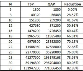
Since in the TSP, only adjacent pairs can exist, all the elements in the flow matrix expect those in the off-diagonals are 0 and hence a few of the variables are 0. Table 3.1 presents a comparison of the number terms in a QAP and in the TSP formulation after elimination of non-adjacent terms with percentage reduction.
Table 3.1: Percentage reduction in the number of variables from QAP to TSP
Linear Assignment Problems (LAP) serve as sub-problems to the TSP and hence the TSP-RLT2 can be solved as a set of LAPs using the parallelized Hungarian Dual ascent algorithm with a branch-and-bound scheme. In the RLT2 phase, we consider a triplet comprising of 3 cities with altleast two of them adjacent. The picture below depicts different ways of forming a triplet in the Z - LAP matrices containing at least one adjacent pair. Consider an ncity problem. In Fig. 3.1a, consider the triplet 1−2−4−p−q −r where 1, 2 and 4 represent the sequence of travel and p, q, r the cities. Since there exists at least one consecutive pair p−q traveled at 1 - 2, this is a validZ(z124pqr) variable. Fig. 3.1b is not a valid triplet because it does not have an adjacent pair.
Therefore, the variable is removed from the Z - LAP and thus the LAP becomes asymmetric with the number of rows in the matrix being either 3, 4 or (n−2) depending on the position of the adjacent pair in the triplet with the column size (n−2).
Figure 3.1: Travel location and its position for TSP
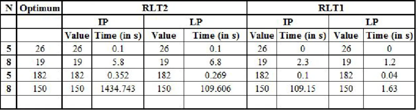
To test our formulation, we ran a few tests on Java - Gurobi environment for instances N = 5 and N = 8. Table 3.2 presents the problem size, optimal objective values obtained from the IP and LP formulations and the solution time for both RLT1 and RLT2. Though the solution time varies, the values obtained from the Integer programming formulation and the relaxed formulation are equal, thus proving the tightness of our TSP-RLT2 formulation.
Table 3.2: Comparison of Integer vs Linear Programming formulation
Date [1] developed a GPU-based Lagrangian Dual Ascent to obtain lower bounds on the QAP-RLT2 and solved the LAPs using a parallel branch-and-bound scheme. The sizes of LAPs due to our TSP formulation is reduced due to the elimination of Z terms with no adjacent pair of cities and hence results in asymmetry. Therefore, we used a modified version of the accelerated Hungarian Algorithm to solve n2(n−1)2 m x n matrices. Next chapter explains in detail the approach to solving our TSP-RLT2.
Chapter 4
Solution Approach
Though RLT2 proves to provide stronger bounds to the LP relaxations, most primal methods fail for large QAP owing to the large number of variables and constraints. Gilmore and Lawler bounds were well-known to provide strong bounds to the LP. Burkard and Stratmann (1978), Edwards (1980), Li et al. (1992) and others provide reduction strategies to obtain lower bounds. Carraresi and Malucelli [63] provided three families of lowers bounds. One: An iterative procedure is used to obtain a suboptimal dual solution by solving the LP without symmetric constraints and interchanging the reduced costs with the symmetric variables. The dual multiplier associated with the symmetric constraint is increased by a quantity equal to the reduced cost, and hence, the process yields a non-decreasing sequence of lower bounds and is repeated till a stopping criterion is reached. In the other two families of lower bounding procedures, a lower bound is computed using the iterative steps mentioned above and dual ascent strategy or the graph-theoretic strategy is applied to strengthen bounds. Adams and Johnson developed a Lagrangian dual ascent scheme and Hahn and Grant furthered this with an augmented dual ascent method with simulated annealing (1998). Adams et al. [56] used the Lagrangian dual ascent to obtain bounds for RLT2 QAP. Hahn et al. (2012) recently proposed a dual ascent based algorithm to find stronger lower bounds on RLT2 and RLT3.
Drawing upon these contributions, in this chapter we propose a solution approach for the TSP. Simply stated, it is a dual ascent procedure for the lower bound of the TSP-RLT2.
4.1
Dual Ascent
Every LP formulation exists in another unique linear programming form called the Dual and can be considered as the inverse of the original formulation, Primal. In other words, if the primal formulation isminf(x), then in the dual space, the objective becomesmaxF(y) such that F(y)≥
f(X) for all feasiblex andy. This implies that if one of them, primal or dual, is feasible, the other cannot be unbounded and if one of them is unbounded, the other will be infeasible. A dual solution can be used to check for optimality; if there is exists an x and y such that f(x) =F(y), then x is the optimal of the primal andy, the dual optimal. Weak duality is when a feasible solution to the dual corresponds to an upper bound on a primal solution. In strong duality, we can guarantee that the optimal solutions to the primal and dual are always equal. Many algorithms use this concept of strong and weak duality and one of them is the Lagrangian Duality.
P : min cx; s.t. Ax≥b; x∈X (4.1)
A simple minimization (P1) has a simple constraintx∈X and a complicating constraint Ax≥b. A dual multiplier or Lagrangian multiplier associated with the relaxed complicating constraint can be added to the objective, thus obtaining the following Lagrangian relaxation.
LRP(u) : min cx + u(b - Ax), s.t. x∈X (4.2) This relaxation provides a lower bound on the primal and hence the objective is to solve theLP R(u) to find a multiplieru that maximizes the objective function of the Lagrangian dual. Two solution procedures, the Subgradient Search method and Lagrangian Dual Ascent, are the most commonly used for obtaining dual multipliers. Here, we discuss the Lagrangian Dual Ascent scheme since it is used in our work.
4.1.1 Lagrangian Dual Ascent
In the Lagrangian Dual Ascent, the direction of ascent (d) with the best step-size for improve-ment in the objective functionLRP(u) can be estimated at each iteration. For some dual solution (ˆu), find a direction such thatd(b−Ax)>0,∀x∈X(ˆu) which provides the best step-size for max-imum improvement in the objective function. If not, the solution ˆu and the corresponding x can be deemed optimal. However, finding the optimal step-size λ that is non-decreasing while main-taining the feasibility of all solutions is NP-hard. In the Lagrangian dual of RLT2, the direction and step-size for improving the dual objective can be determined without solving the optimization problem but by performing sensitivity analysis while maintaining the complementary slackness for the non-basicx,y andz variables in the corresponding LAPs. In the next section, we will discuss the sequential Hungarian Algorithm and the Lagrangian dual ascent procedure.
4.1.2 Finding the ascent direction and step-size using Langrangian Dual Ascent
The LDRLT2 can be used to find the direction of ascent and the optimal step-size without solving the optimization problem using Lagrangian Dual Ascent. If π(.) denotes the reduced cost
of a variable, for some variable zijkpqr in an optimal LAP solution,
zijkpqr = 1⇒π(zijkpqr) = 0; and zijkpqr = 0⇒π(zijkpqr)≥0 (4.3)
Due to the symmetric constraints, if the TSP solution is optimal, the values of all Z symmetric variables will be the same. If a variable zijkpqr and one of its complementary variableszjikqpr have
contradicting values of 0 and 1, the values (1, - 1) provides a natural direction of ascent and a new dual solution can be obtained by decreasing theDijkpqrby at mostπ(zijkpqr) (increasingvijkpqrˆ ) and
increasing the complementary variable co-efficient Djikqpr using a valid step-size. While choosing
a step -size, the feasibility of the current dual variables α, β, γ, δ, ζ, ψ should be maintained. If the reduced cost π(zijkpqr) < 0, it means there is infeasibility and Dijkpqr should be decreased
by at most π(zijkpqr). Since the complementary variable zjikpqr is basic, this adjustment will
increase (LDRLT2) by some nonnegative value resulting in a strong direction of ascent. If both the complementary variables are 0, i.e., if they are both non-basic, any increase toDijkpqr will not
change (LDRLT2) and is a weak direction of ascent. By finding a strong direction of ascent, we can ensure a non-negative increase in v(LDRLT2). i.e., instead of finding a strong direction for every pair in the symmetric constraint, we can find a strong direction for one of the pairs by selecting a non-basic variable, decreasing its cost by some amount and increasing the cost coefficients of the other five complementary variables by a fraction of it. By doing so, there will be a non-negative increase in the dual and if no strong direction is found, the objective value remains the same.
This has shown to outperform all other bounding schemes. Though solving O(n4) LAPs and updating the O(n6) multipliers can be computationally heavy, the advantage of the RLT2-DA is that each of the LAPs can be solved independently, Therefore, parallelizing this algorithm will ensure faster results. CUDA enabled NVIDIA GPUs is chosen as the primary architecture for the dual update phase of DA. The GPU-accelerated algorithm for LAP together with the RLT2-DA solver are used to speed up the process of solving LAP and to obtain strong lower bounds on the QAP. We use this same procedure described in Date [1] for solving the TSP.
4.2
Hungarian Algorithm
The Hungarian Algorithm was proposed by Kuhn (1955) and is used in problems where an nx nmatrix has every element representing a cost associated with assigning some j-th job/facility to i-th worker/location and the objective of the problem is to find an optimal assignment of the jobs. In each iteration of the Hungarian algorithm, the number of assignments increases or a new edge with slack cij −ui−vj = 0 is obtained. At each step, an adjacency list with the zero slack edges
is stored and modified. Since the matrix containsn2 variables, the process is repeated at mostn2 times and hence the complexity is O(n4)
4.2.1 Sequential Hungarian Algorithm
Consider the dual LP relaxation of the TSP - RLT2 (LRLT2) formulation with relaxed Z symmetric constraints added to the objective using v = ˆvijkpqr and α, β, γ, δ, ζ, ψ representing the
dual variables corresponding to the constraints. DLRLT2(ˆv) : maxX i αi+ X i βp (4.4) s.t. αi+βp− X j6=i γijp− X q6=p δipq ≤bip, ∀i, p (4.5) γijp +δijp− X k6=i,j ζijkpq− X r6=q,p ψijpqr ≤Cijpq, ∀(i6=j, p6=q) (4.6) ζijkpq+ψijpqr ≤Dijkpqr −vˆijkpqr, ∀(i6=j 6=k, p6=q 6=r) (4.7) αi, βp, γijp, δipq, ζijkpq, ψijpqr ∼unrestricted ∀(i6=j 6=k, p6=q 6=r) (4.8)
The problem DLRLT2(ˆv) can be solved in three stages using the decomposition principle proposed by Adams et al. by leveraging the values obtained in the individual stages. To maximize the dual objective w.r.t. (4.7), we need large values of α and β, for which P
j6=i
γijp − P q6=p
δipq
needs to be maximized subject to (4.8). Subsequently, this requires large values of γ and δ, which requires maximization of P
k6=i,j
ζijkpq− P r6=q,p
ψijpqr w.r.t. (4.9), which constitutes the first stage of the problem. We solve each of these in its dual form: first solven2(n−1)2 Z - LAPs, then we solve n2 Y - LAPs and finally the X - LAP which will gives us the required lower bound. Thus, we solve O(n4) LAPs andO(n2) cost coefficients in each LAP. At each of the three stages, an alternating tree version of the Hungarian Algorithm is used to solve the LAPs. The algorithm tries to find maximum matching subject to condition(Dijkpqr−vˆijkpqr−ζijkpq−ψijpqr)∗Zijkpqr = 0. If the slack (Dijkpqr −vˆijkpqr−ζijkpq −ψijpqr) = 0,Zijkpqr can be set to 1, which means the tourp−q−rin the order i−j−kis fixed. If not, dual variables are adjusted to introduce one new city into the tour with 0 slack using the dual ascent procedure. First, using reduction, a minimum non - zero slack is identified and the dual multipliers are updated. Then, the LAPs are resolved to obtain an improved solution for LP relaxation of RLT2. Using the complementary slackness condition, the primal-dual feasibility check is performed. The process of solving the LAP and dual ascent is alternated till an optimal solution is found. In our solution framework, we use a modified version of the GPU-accelerated Hungarian algorithm for the Linear Assignment Problem proposed by Ketan Date and Rakesh Nagi [64].
Ascent and Parallelizations.
4.3
Accelerating RLT2-DA Algorithm for the TSP Using a GPU
Cluster
This section looks at the solution approach for the TSP in its entirety. The LAP matrices / cost coefficients are split across multiple GPUs and a grid architecture with multiple processing units, each with a CPU - GPU pair is used in solving several LAPs. Each of the k GPUs perform a set of functions simultaneously:
Initialization → Dual Ascent → Z-TLAP Solve → Y-TLAP Solve → X-LAP
Solve → Feasibility Check
1. Initialization
The first in the process is to initialize the program with k MPI processes, with each MPI process assigned to one CPU and each GPU has equal number of LAPs i.e., the cost matrices for the Y and Z LAPs are split evenly across all the
n2(n−1)2
K
Z-LAP matrices and n2
K
Y-LAP matrices and the root GPU owns the X-LAP matrix.
2. Dual Ascent
This step is parallelized by simply assigning each thread of the GPU to a multiplier associated with one z-variable of the LAP on the GPU and a host of multipliers are updated at once. At each iteration of the RLT2-DA step, the cost co-efficients b0, C0, D0 are updated using MPI to transfer the array of dual variables and the modified cost matrices between CPUs and GPUs.
3. LAP Solution
The X - LAP is of sizen×nand each of then2 Y LAPs are of size(n−1)×(n−1). All the Y - LAPs and the X - LAP are solved using the alternating-tree variant of accelerated Hungarian algorithm and a modified version of the tiled LAP solver is used to solve the asymmetric Z - LAPs. To leverage the efficiency of the GPU-accelerated algorithm, the LAPs are tiled and solved instead of solving them individually. For example, if there areMY Y-LAP matrices on a particular GPU, then instead of solving them one at a time, all of them are solved as a single TLAP since it is
known to solve faster than a single LAP though the complexity isO(M1.5n3), worse as compared toO(M n3).
4.4
Computational Experiments
In this section, we present our computational results. We compare the two TSP representations, a full QAP representation and its reduced form without non-adjacent variables, for its solution times.
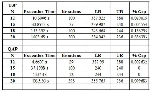
Table 4.1: Comparison of Solution times of QAP and reformulated TSP
Table 4.1 reports the results for RANDOM instances. The algorithm is terminated if the gap in a particular iteration is < 1% or if it reaches the number of iterations specified, whichever is earlier. Our point of concentration is the execution times. The problem size (N) is presented in the first column. For problem sizes <18, we tested on a single GPU and for larger problem instances, we used 2 GPUs due to increase in memory requirements. We can see that, for a given number or iterations, the lower bounds are almost the same for both the formulations and the gap remains less than1%implying that the formulation is tight. We see that the solution times for our TSP-RLT2 reduces by half as compared to the QAP representation of the TSP.
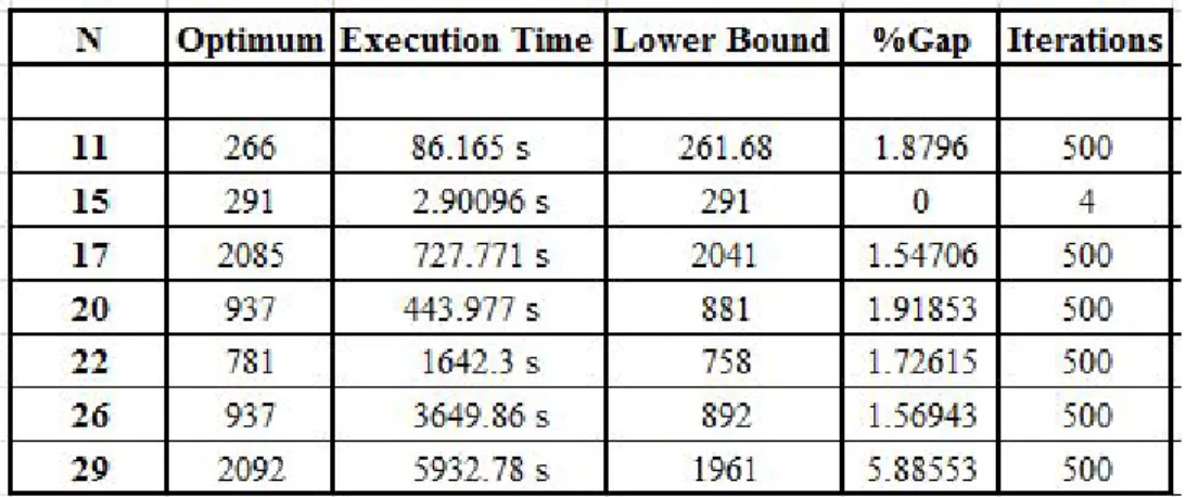
Table 4.2 gives insights about the solution times and bounds for standard TSP instances. The lower bounds obtained were nearly optimum to values obtained from [65]. This is an affirmation of the fact that our model provides tight lower bounds and low % gaps. For problem instance N = 29, the QAP model could not be solved using 2 cards owing to its large size and can be handled by increasing either the number of GPUs or CPUs.
Table 4.2: Solution times for instances from TSPLIB TSP
and Table 4.3 presents the results. The restriction in the RLT2 approach is the need for symmetry in either the flow matrix or distance matrix. Since we have a symmetric flow matrix, our formulation is indifferent to Symmetric and Asymmetric TSPs and the results presented in this table shows performance to be independent of the kind of TSP and is mostly instance specific. Numerical analysis may be performed to reinstate the performance efficiency of our solver for Symmetric and Asymmetric problems.
Table 4.3: Comparison of Solution times for a Symmetric v/s Asymmetric TSP
The Hungarian Algorithm with RLT2 - Dual Ascent is computational demanding for the Trav-eling Salesman Problem. Yet, the bounds obtained due to the dual ascent approach are extremely tight for most problems from the TSPLIB with problem size N < 30. When ported to a GPU clustered environment with 2 nodes and 4 devices, larger problems can be solved.
Chapter 5
Conclusions
In review, we reformulated a Quadratic Assignment Problem as a Traveling Salesman Prob-lem and applied a Level-2 Reformulation Linearization Technique to overcome the complexities of quadratic objective function. We solved this reformulated TSP on an LAP solver with alternat-ing tree variant of the Hungarian Algorithm and used a Graphics Processalternat-ing Units (GPU) based version of the Lagrangian dual ascent procedure (RLT2-DA) for obtaining lower bounds. The pro-cedure involved two steps: After initializations, using the parallelized GPU-accelerated Hungarian algorithm, we solve a bunch of LAPs independent of each other and in the second step we update dual multipliers using Dual Ascent.
A comparison between the solution times of TSP as a full QAP matrix using Hungarian algo-rithm and that of the TSP as a reduced QAP was made. The reduction in solution times for our reformulated TSP model was reduced by half for a given number of iterations. The lower bounds obtained were tight and the %gap was fairly small. Due to computational restrictions, we could only test small instances with problem size N < 30, but larger problem sizes can be solved by using a multi-CPU cluster.
Bibliography
[1] Ketan Hemant Date. Theoretical and computational advances in finite-size facility placement and assignment problems. http://hdl.handle.net/2142/95355, 2016.
[2] Abraham P Punnen and Gregory Gutin. Traveling Salesman Problem and Its Variations (Combinatorial optimization; v. 12). Springer, 2007.
[3] George Dantzig, Ray Fulkerson, and Selmer Johnson. Solution of a large-scale traveling-salesman problem. Journal of the operations research society of America, 2(4):393–410, 1954. [4] G Morton and AH Land. A contribution to the” travelling-saleman” problem. Journal of the
Royal Statistical Society. Series B (Methodological), pages 185–203, 1955.
[5] LL Barachet. Letter to the editor-graphic solution of the traveling-salesman problem. Opera-tions Research, 5(6):841–845, 1957.
[6] ML Balinski and RE Gomory. A primal method for the assignment and transportation prob-lems. Management Science, 10(3):578–593, 1964.
[7] Richard Bellman. Dynamic programming and lagrange multipliers. Proceedings of the National Academy of Sciences, 42(10):767–769, 1956.
[8] John DC Little, Katta G Murty, Dura W Sweeney, and Caroline Karel. An algorithm for the traveling salesman problem. Operations research, 11(6):972–989, 1963.
[9] P Miliotis. Using cutting planes to solve the symmetric travelling salesman problem. Mathe-matical programming, 15(1):177–188, 1978.
[10] Clair E Miller, Albert W Tucker, and Richard A Zemlin. Integer programming formulation of traveling salesman problems. Journal of the ACM (JACM), 7(4):326–329, 1960.
[11] Hanif D. Sherali and Patrick J. Driscoll. On tightening the relaxations of miller-tucker-zemlin formulations for asymmetric traveling salesman problems.Operations Research, 50(4):656–669, 2002.
[12] Wong RT. Integer programming formulations of the traveling salesman problem. Proceedings of the IEEE international conference of circuits and computers, pages 149–52, 1980.
[13] Moustapha Diaby. The traveling salesman problem: a linear programming formulation. arXiv preprint cs/0609005, 2006.
[14] Anja Fischer, Frank Fischer, Gerold J¨ager, Jens Keilwagen, Paul Molitor, and Ivo Grosse. Ex-act algorithms and heuristics for the quadratic traveling salesman problem with an application in bioinformatics. Discrete Applied Mathematics, 166:97–114, 2014.
[15] Borzou Rostami, Federico Malucelli, Pietro Belotti, and Stefano Gualandi. Lower bounding procedure for the asymmetric quadratic traveling salesman problem. European Journal of Operational Research, 253(3):584–592, 2016.
[16] Moustapha Diaby, Mark H Karwan, and Lei Sun. A small-order-polynomial-sized linear pro-gram for solving the traveling salesman problem. arXiv preprint arXiv:1610.00353, 2016. [17] Merrill M Flood. The traveling-salesman problem. Operations Research, 4(1):61–75, 1956. [18] Harold W Kuhn. Variants of the hungarian method for assignment problems. Naval Research
Logistics Quarterly, 3(4):253–258, 1956.
[19] RH Mole, DG Johnson, and K Wells. Combinatorial analysis for route first-cluster second vehicle routing. Omega, 11(5):507–512, 1983.
[20] Daron Roberts and E Hadjiconstantinou. Algorithmic developments in stochastic vehicle rout-ing. InOperations Research Proceedings 1997, pages 156–161. Springer, 1998.
[21] Tolga Bektas. The multiple traveling salesman problem: an overview of formulations and solution procedures. Omega, 34(3):209–219, 2006.
[22] Gilbert Laporte and Yves Nobert. A cutting planes algorithm for the m-salesmen problem.
Journal of the Operational Research society, 31(11):1017–1023, 1980.
[23] Bezalel Gavish and Kizhanathan Srikanth. An optimal solution method for large-scale multiple traveling salesmen problems. Operations Research, 34(5):698–717, 1986.
[24] J Gromicho, J Paix˜ao, and I Bronco. Exact solution of multiple traveling salesman problems. InCombinatorial Optimization, pages 291–292. Springer, 1992.
[25] Sneˇzana Mitrovi´c-Mini´c and Ramesh Krishnamurti. The multiple tsp with time windows: vehicle bounds based on precedence graphs. Operations Research Letters, 34(1):111–120, 2006. [26] RA Russell. Effective heuristic for m-tour traveling salesman problem with some side con-ditions. In Operations Research, volume 23, pages B296–B296. Inst. Operations Research Management Sciences 901 Elkridge Landing Rd, Ste 400, Linthicum HTS, MD 21090-2909, 1975.
[27] Shen Lin and Brian W Kernighan. An effective heuristic algorithm for the traveling-salesman problem. Operations research, 21(2):498–516, 1973.
[28] David B Fogel. A parallel processing approach to a multiple traveling salesman problem using evolutionary programming. In Proceedings of the fourth annual symposium on parallel processing, pages 318–326. Fullerton, CA, 1990.
[29] Chau-Yun Hsu, Meng-Hsiang Tsai, and Wei-Mei Chen. A study of feature-mapped approach to the multiple travelling salesmen problem. InCircuits and Systems, 1991., IEEE International Sympoisum on, pages 1589–1592. IEEE, 1991.
[30] Abdolhamid Torki, Samerkae Somhon, and Takao Enkawa. A competitive neural network algorithm for solving vehicle routing problem. Computers & industrial engineering, 33(3):473– 476, 1997.
[31] Abdolhamid Modares, Samerkae Somhom, and Takao Enkawa. A self-organizing neural net-work approach for multiple traveling salesman and vehicle routing problems. International Transactions in Operational Research, 6(6):591–606, 1999.
[32] Samerkae Somhom, Abdolhamid Modares, and Takao Enkawa. Competition-based neural network for the multiple travelling salesmen problem with minmax objective. Computers & Operations Research, 26(4):395–407, 1999.
[33] Tiehua Zhang, WA Gruver, and Michael H Smith. Team scheduling by genetic search. In
Intelligent Processing and Manufacturing of Materials, 1999. IPMM’99. Proceedings of the Second International Conference on, volume 2, pages 839–844. IEEE, 1999.
[34] Lixin Tang, Jiyin Liu, Aiying Rong, and Zihou Yang. A multiple traveling salesman problem model for hot rolling scheduling in shanghai baoshan iron & steel complex. European Journal of Operational Research, 124(2):267–282, 2000.
[35] Zhong Yu, Liang Jinhai, Gu Guochang, Zhang Rubo, and Yang Haiyan. An implementation of evolutionary computation for path planning of cooperative mobile robots. In Intelligent Control and Automation, 2002. Proceedings of the 4th World Congress on, volume 3, pages 1798–1802. IEEE, 2002.
[36] Joel L Ryan, T Glenn Bailey, James T Moore, and William B Carlton. Reactive tabu search in unmanned aerial reconnaissance simulations. InProceedings of the 30th conference on Winter simulation, pages 873–880. IEEE Computer Society Press, 1998.
[37] Chi-Hwa Song, Kyunghee Lee, and Won Don Lee. Extended simulated annealing for augmented tsp and multi-salesmen tsp. In Neural Networks, 2003. Proceedings of the International Joint Conference on, volume 3, pages 2340–2343. IEEE, 2003.
[38] Gilbert Laporte and Yves Nobert. Generalized travelling salesman problem through n sets of nodes: An integer programming approach. INFOR: Information Systems and Operational Research, 21(1):61–75, 1983.
[39] Gilbert Laporte, H´el`ene Mercure, and Yves Nobert. Generalized travelling salesman problem through n sets of nodes: the asymmetrical case. Discrete Applied Mathematics, 18(2):185–197, 1987.
[40] Matteo Fischetti, Juan Jos´e Salazar Gonz´alez, and Paolo Toth. A branch-and-cut algorithm for the symmetric generalized traveling salesman problem. Operations Research, 45(3):378–394, 1997.
[41] Charles E Noon and James C Bean. A lagrangian based approach for the asymmetric gener-alized traveling salesman problem. Operations Research, 39(4):623–632, 1991.
[42] Charles E Noon and James C Bean. An efficient transformation of the generalized traveling salesman problem.INFOR: Information Systems and Operational Research, 31(1):39–44, 1993. [43] AG Chentsov and LN Korotayeva. The dynamic programming method in the generalized
traveling salesman problem. Mathematical and Computer Modelling, 25(1):93–105, 1997. [44] David Ben-Arieh, Gregory Gutin, M Penn, Anders Yeo, and Alexey Zverovitch.
[45] Boris Bontoux, Christian Artigues, and Dominique Feillet. A memetic algorithm with a large neighborhood crossover operator for the generalized traveling salesman problem. Computers & Operations Research, 37(11):1844–1852, 2010.
[46] Gregory Gutin and Daniel Karapetyan. A memetic algorithm for the generalized traveling salesman problem. Natural Computing, 9(1):47–60, 2010.
[47] Daniel Karapetyan and Gregory Gutin. Lin–kernighan heuristic adaptations for the generalized traveling salesman problem.European Journal of Operational Research, 208(3):221–232, 2011. [48] Chi-Bin Cheng and Chun-Pin Mao. A modified ant colony system for solving the travelling salesman problem with time windows. Mathematical and Computer Modelling, 46(9):1225– 1235, 2007.
[49] Roberto Wolfler Calvo. A new heuristic for the traveling salesman problem with time windows.
Transportation Science, 34(1):113–124, 2000.
[50] Jeffrey W Ohlmann and Barrett W Thomas. A compressed-annealing heuristic for the traveling salesman problem with time windows. INFORMS Journal on Computing, 19(1):80–90, 2007. [51] Jing-Quan Li. A bi-directional resource-bounded dynamic programming approach for the
traveling salesman problem with time windows. Submitted manuscript.
[52] John N Tsitsiklis. Special cases of traveling salesman and repairman problems with time windows. Networks, 22(3):263–282, 1992.
[53] Kjetil Fagerholt and Marielle Christiansen. A travelling salesman problem with allocation, time window and precedence constraintsan application to ship scheduling. International Transac-tions in Operational Research, 7(3):231–244, 2000.
[54] Norbert Ascheuer, Matteo Fischetti, and Martin Gr¨otschel. Solving the asymmetric travel-ling salesman problem with time windows by branch-and-cut. Mathematical Programming, 90(3):475–506, 2001.
[55] Vicky Mak and Andreas T Ernst. New cutting-planes for the time-and/or precedence-constrained atsp and directed vrp.Mathematical Methods of Operations Research, 66(1):69–98, 2007.
[56] Warren P Adams, Monique Guignard, Peter M Hahn, and William L Hightower. A level-2 reformulation–linearization technique bound for the quadratic assignment problem. European Journal of Operational Research, 180(3):983–996, 2007.
[57] Tjalling C Koopmans and Martin Beckmann. Assignment problems and the location of eco-nomic activities. Econometrica: journal of the Econometric Society, pages 53–76, 1957. [58] Eugene L Lawler. The quadratic assignment problem. Management science, 9(4):586–599,
1963.
[59] AM Frieze and J Yadegar. On the quadratic assignment problem. Discrete applied mathemat-ics, 5(1):89–98, 1983.
[60] Warren P Adams and Hanif D Sherali. A tight linearization and an algorithm for zero-one quadratic programming problems. Management Science, 32(10):1274–1290, 1986.
[61] Warren P Adams and Terri A Johnson. Improved linear programming-based lower bounds for the quadratic assignment problem. DIMACS series in discrete mathematics and theoretical computer science, 16:43–75, 1994.
[62] Nicos Christofides and Enrique Benavent. An exact algorithm for the quadratic assignment problem on a tree. Operations Research, 37(5):760–768, 1989.
[63] Paolo Carraresi and Federico Malucelli. A new lower bound for the quadratic assignment problem. Operations Research, 40(1-supplement-1):S22–S27, 1992.
[64] Ketan Date and Rakesh Nagi. Gpu-accelerated hungarian algorithms for the linear assignment problem. Parallel Computing, 57:52–72, 2016.