Published online in Wiley InterScience (www.interscience.wiley.com). DOI: 10.1002/acs
Highly computationally efficient state filter based on the delta
operator
Xiao Zhang
1, Feng Ding
∗1,2, Ling Xu
1and Erfu Yang
31 Key Laboratory of Advanced Process Control for Light Industry (Ministry of Education), School of Internet of Thiings Engineering, Jiangnan University, Wuxi 214122, PR China
2 College of Automation and Electronic Engineering, Qingdao University of Science and Technology, Qingdao 266061, PR China
3 Space Mechatronic Systems Technology Laboratory, University of Strathclyde, Glasgow G1 1XJ, Scotland, United Kingdom
SUMMARY
The Kalman filter is not suitable for the state estimation of linear systems with multi-state-delays and the extended state vector Kalman filtering algorithm results in heavy computational burden because of the large dimension of the state estimation covariance matrix. Thus, in this paper, we develop a novel state estimation algorithm for enhancing the computational efficiency based on the delta operator. The computation analysis and the simulation example show the performance of the proposed algorithm. Copyright c°2018 John Wiley & Sons, Ltd.
Received . . .
KEY WORDS: Time-delay system, Kalman filtering, state estimation, delta operator
1. INTRODUCTION
As the basis of modern control theory, the state-space representation is an effective mathematical model to totally describe the dynamic behaviors of physical systems [1]. Compared with the transfer function representation [2,3,4], it can be applied to more complex systems such as multi-input multi-output systems [5] and nonlinear systems [6]. Filtering methods have been widely used in parameter estimation [7,8], and the combined state and parameter estimation of state-space systems have attracted much attention throughout the world [9]. Sch¨on studied an expectation maximization algorithm for nonlinear systems described by state-space models and acquired the state estimates through a particle smoother [10]. Partovibakhsh and Liu proposed an adaptive unscented Kalman filtering based approach for jointly online estimation of state-of-charge and parameters of lithium-ion batteries for autonomous mobile robots and computed the noise covariances in the state estimation process by covariance matching [11].
Time delays often exist in signal transmission and signal modeling [12-16] and control systems [17,18,19]. For example, in communication, the measurements are often obtained with time delay because of the transmission congestion; the communication networks between subsystems are often unreliable, which will introduce the communication delays. Some important variables of chemical processes are often obtained through online analyzers, resulting large time delays [20].Such delays may cause instability and poor performance of system dynamics [21]. Thus the analysis and control
∗Correspondence to: Key Laboratory of Advanced Process Control for Light Industry, School of Internet of Thiings
Engineering, Jiangnan University, Wuxi 214122, China.
of time-delay systems are imporatnt [22]. In the literature, Chen et al. utilized a biased compensation recursive least squares algorithm to estimate the parameters and delays of a time-delay rational model [23]. Shi et al. considered the state estimation of Markovian jump neural networks with time-delays, and developed a state estimator to obtain the network state estimates for the error dynamics to be stochastic finite-time stable [24].Xu utilized the first-order Taylor expansion to approximate the time delay and presented a proportional differential control algorithm for parameter estimation of first-order time-delay model with transfer function [25]. Gu et al. presented an iterative based identification algorithm for linear models with multi-state-delays based on the negative gradient search and the least squares principle, but without considering the state estimation of the unknown states [26]. To the best of our knowledge, the related work has not been reported in the literature on the state estimation of dynamic systems with multi-state-delays. Thus, there is a strong incentive for us to develop an efficient state filter of such systems.
Parameter estimation and state filtering are basic for system identification [27,28,29] and system analysis and design [30,31,32,33], and can be applied to many areas [34-39]. The Kalman filter (KF) is known as the optimal state filter for linear systems under the Gussian white noise and has been extended to study the parameter estimation for bilinear systems [40,41,42]. For nonlinear systems, its modifications such as the particle filter, the extended Kalman filter, the unscented Kalman filter give approaches for nonlinear filtering problems. Differing from the above state filters in the recursive way, Zhao et al. developed an unbiased finite impulse response filter to iteratively estimate the state variables using a fixed number of recent measurements [43]. Shi et al. presented a Kalman filter based parameter estimation algorithm on the basis of an output estimator for networked control systems with missing output data and designed an adaptive controller to achieve the output tracking [44].
The KF is employed to provide solutions for the state estimation of the linear system with multi-state-delays. However, according to the computational analysis (see in Section 3), the dimension of the state estimation covariance matrix is large, which causes the high computational burden for state estimation. This motivates us to search for a highly-computationally-efficient state estimation algorithm with high computational efficiency for estimating the system state based on the knowledge of system dynamics and noisy observation data.The main contributions of this paper are as follows.
• Study a highly-computationally-efficient state filter for a multi-time-delay system described by a state-space model.
• Apply the delta operator to minimize the state estimation error covariance matrix, resulting in the improvement of computational efficiency.
• Analyze the computational complexity between the presented algorithms to demonstrate the performance of the state filter based on the floating point operation.
The paper is organized as follows. Section2formulates the problem and presents a generalized state estimation algorithm by gathering the sub-vectors into an extended state vector. Then a direct state estimation algorithm based on the delta operator is presented to reduce the computational burden in Section3. The benefits of the proposed methods are shown by the simulation examples in Section4. Finally, Section5provides some concluding remarks.
2. THE PROBLEM FORMULATION Some necessary symbols are introduced as follows.
Symbols Meaning
A=:X Xis defined byA.
X :=A Xis defined byA.
1n Ann-dimensional column vector whose
entries are all 1. E[x] The expectation ofx.
I An identity matrix of appropriate size (n×n).
z A unit forward shift operator like
zx(s) =x(s+ 1)andz−1x(s) =x(s−1).
T The vector/matrix transpose.
For the state-space system with a unit time-delay, there are some methods for discussing its stability and identification problems [45,46]. For more general conditions, this paper considers a linear system with multi-time-delays:
x(s+ 1) =Ax(s) +B1x(s−1) +B2x(s−2) +· · ·
+Brx(s−r) +bu(s) +w(s), (1)
y(s) =cx(s) +v(s), (2)
whereu(s)∈Rdenotes the sampled input,y(s)∈Ris the system output disturbed by a stochastic noisev(s),x(s)∈Rnis the state vector,w(s)∈Rn is the process noise,A∈Rn×n,B
q∈Rn×n
(q= 1,2, . . . , r),b∈Rnandc∈R1×nare the system parameters.
Assume that the system output variable is disturbed by a stochastic noisev(s)with zero mean and varianceRv,w(s)∈Rn is the uncorrected process noise vector with zero mean and variance
Rw. The noisesw(s)andv(s)are uncorrelated and their covariance matrices satisfy
(A1) E[w(s)] =0, E[v(s)] = 0, E[w(s)v(i)] =0,
(A2) E[w(s)wT(s)] =0, E[v(l)v(t)] = 0, l6=t, (A3) E[w(s)wT(s)] =R
w∈Rn×n,E[v2(s)] =Rv ∈R.
Assume that the system in (1)–(2) is stable, observable and controllable. For a linear dynamic system with multi-state-delays, the Kalman filter cannot be employed directly to obtain the optimal state estimates. Here we present a generalized state estimation algorithm on the basis of the Kalman filter to compute the estimates of the unknown states.
Define the extended state vector X(s) := [xT(s),xT(s−1),xT(s−2),· · · ,xT(s−r)]T∈
Rnr+n and the extended noise vectorW(s) := [wT(s),0,· · ·,0]T∈Rnr+n. Then System (1)–(2)
can be expressed as
X(s+ 1) =GX(s) +Hu(s) +W(s), (3)
y(s) =Γ X(s) +v(s), (4)
where the parameter matrices and vectors are defined as
G:= A B1 B2 · · · Br In 0 0 · · · 0 0 In 0 . .. ... .. . . .. ... ... 0 0 · · · 0 In 0 ∈R(nr+n)×(nr+n), H:= [bT,0,0,· · ·,0]T∈Rnr+n, Γ := [c,0,0,· · · ,0]∈R1×(nr+n).
For the state vector X(s), it is well-known that the Kalman filter can be employed to estimate the unknown states for the linear systems from observation data. Let Xˆ(s|s−1)∈Rnr+n and
ˆ
X(s|s)∈Rnr+n be the predicted state estimate and the posterior state estimate of the unknown
X(s). LetK(s)∈Rnr+ndenote the optimal gain vector,P(s|s−1)∈R(nr+n)×(nr+n)denote the
priori state estimation error covariance matrix of X(s)andP(s|s)∈R(nr+n)×(nr+n) denote the
posteriori state estimation error covariance matrix ofX(s). Based on the Kalman filtering principle, we obtain the generalized state estimation algorithm:
ˆ
X(s|s) = ˆX(s|s−1) +K(s)[y(s)−ΓXˆ(s|s−1)], (5)
K(s) =P(s|s−1)ΓT[Γ P(s|s−1)ΓT+R
P(s|s) = [I−K(s)Γ]P(s|s−1)[I−K(s)Γ]T+K(s)R vKT(s), (7) ˆ X(s|s−1) =GXˆ(s−1|s−1) +Hu(s−1), (8) P(s|s−1) =GP(s−1|s−1)GT+R W. (9)
Define the state estimateXˆ(s) := ˆX(s|s)ofX(s) at timesand the covariance matrixP(s) :=
P(s|s)at times. Then through eliminating the intermediate variablesX(s|s−1)andP(s|s−1) in (5) to (9), we obtain the generalized Kalman filtering algorithm:
ˆ X(s) =GXˆ(s−1) +Hu(s−1) +K(s){y(s)−Γ[GXˆ(s−1) +Hu(s−1)]}, (10) K(s) = [GP(s−1)GT+R W]ΓT{Γ[GP(s−1)GT+RW]ΓT+Rv}−1, (11) P(s) = [I−K(s)Γ][GP(s−1)GT+R W][I−K(s)Γ]T+K(s)RvKT(s). (12)
Remark 1. Although the state estimation algorithm in (10)–(12) can be directly derived based on the Kalman filtering principle, the most remarkable problem is its heavy computational burden, especially for large-scale systems.
Remark 2. Because of the existence of the multi-state-delays, the dimension of the state-space model sharply increases, which makes the dimension of the extended state vector become quite large and causes heavy computational burden. This motivates us to design a highly-efficient state filter for state estimation of the dynamics system with multi-state-delays from noisy observation data.
The objective of this paper is to develop a highly-efficient state estimation algorithm based on the delta operator. This method avoids gathering the sub-state vectors into an extended state vector
X(s)and greatly improves the computational efficiency – see TableIII.
3. THE DIRECT STATE ESTIMATION ALGORITHM BASED ON THE DELTA OPERATOR In order to improve the computational efficiency, this section presents a direct state estimation algorithm in a two-step process for the linear system in (1)–(2).
Let xˆo(s+ 1) := ˆx(s+ 1|s) denote the predicted state estimate of x(s+ 1) based on the
observation data up to time s+ 1, and xˆ(s+ 1) := ˆx(s+ 1|s+ 1) denote the posteriori state estimate ofx(s+ 1)based on the observation data up to and including times+ 1.
Prediction Step:The predicted state, i.e., the open-loop state estimate can be expressed as ˆ
xo(s+ 1) =Axˆ(s) +B1xˆ(s−1) +B2xˆ(s−2) +· · ·+Brxˆ(s−r) +bu(s). (13)
Define the priori state error covariance matrix as
Po(s) := E{[x(s)−xˆo(s)][x(s)−xˆo(s)]T} ∈Rn×n.
ThenPo(s+ 1)can be computed by
Po(s+ 1) = E{[x(s+ 1)−xˆo(s+ 1)][x(s+ 1)−xˆo(s+ 1)]T} = E{[Ax(s) +B1x(s−1) +· · ·+Brx(s−r) +bu(s) +w(s)−Axˆ(s)−B1xˆ(s−1) −B2xˆ(s−2)− · · · −Brxˆ(s−r)−bu(s)][Ax(s) +B1x(s−1) +B2x(s−2) +· · ·+Brx(s−r) +bu(s) +w(s)−Axˆ(s)−B1xˆ(s−1) −B2xˆ(s−2)− · · · −Brxˆ(s−r)−bu(s)]T} = E{[Ae(s) +B1e(s−1) +B2e(s−2) +· · · +Bre(s−r) +w(s)][Ae(s) +B1e(s−1) +B2e(s−2) +· · ·+Bre(s−r) +w(s)]T}. (14)
Update Step: Once the new measurement data u(s+ 1) andy(s+ 1) are sampled, the modified state estimate, i.e., the closed-loop state estimate can be expressed as
ˆ
x(s+ 1) = ˆxo(s+ 1) +K(s+ 1)[y(s+ 1)−cxˆo(s+ 1)]
=Axˆ(s) +B1xˆ(s−1) +B2xˆ(s−2) +· · ·
+Brxˆ(s−r) +bu(s) +K(s+ 1)
×[cx(s+ 1) +v(s+ 1)−cxˆo(s+ 1)], (15)
whereK(s+ 1)is the state gain vector.
Remark 3: The choice ofK(s+ 1)determines the weight of the predicted statexˆo(s+ 1)and the
practical measurement datay(s+ 1)when updating the state estimatexˆ(s+ 1).
Define the state error ase(s) :=x(s)−xˆ(s)∈Rn, and the posteriori covariance matrix as
P(s) := E{[x(s)−xˆ(s)][x(s)−xˆ(s)]T}
= E{e(s)eT(s)} ∈Rn×n. (16)
Then the state estimation error covariance matrixP(s)can be calculated by
P(s+ 1) = E{[x(s+ 1)−xˆ(s+ 1)][x(s+ 1)−xˆ(s+ 1)]T} = E{[Ae(s) +B1e(s−1) +B2e(s−2) +· · · +Bre(s−r) +w(s)−K(s+ 1)c[x(s+ 1) −xˆo(s+ 1)]−K(s+ 1)v(s+ 1)][Ae(s) +B1e(s−1) +B2e(s−2) +· · ·+Bre(s−r) +w(s)−K(s+ 1)c ×[x(s+ 1)−xˆo(s+ 1)]−K(s+ 1)v(s+ 1)]T = E{{[I−K(s+ 1)c][x(s+ 1)−xˆo(s+ 1)] −K(s+ 1)v(s+ 1)}{[I−K(s+ 1)c][x(s+ 1) −xˆo(s+ 1)]−K(s+ 1)v(s+ 1)}T} = [I−K(s+ 1)c]Po(s+ 1)[I−K(s+ 1)c]T +K(s+ 1)RvKT(s+ 1). (17)
Because the system statex(s), and the state estimatesxˆ(s)andxˆo(s)are uncorrected withw(s).
That is to say,E{x(s)wT(s)}=0,E{xˆ(s)wT(s)}=0,E[e(s−i)wT(s)] =0(i= 0,1,2, . . . , r). From (14), we have Po(s+ 1) =AE{e(s)eT(s)}AT+B1E{e(s−1)eT(s−1)}B1T+· · · +BrE{e(s−r)eT(s−r)}BTr+AE{e(s) ×eT(s−1)}BT 1+· · ·+AE{e(s)eT(s−r)}BrT +B1E{e(s−1)eT(s)}AT+· · ·+B1E{e(s−1) ×eT(s−r)}BT r+BrE{e(s−r)eT(s)}AT+· · · +BrE{e(s−r)eT(s−r+ 1)}Br−T 1+ E{w(s)wT(s)}. (18)
Define the covariance matrixPij(s) := E[e(s−i)e(s−j)],i= 0,1,2, . . . , r,j= 0,1, . . . , r. Then
Po(s+ 1)can be expressed as
Po(s+ 1) = [A,B1,B2, . . . ,Br]P1(s)[A,B1,B2, . . . ,Br]T+Rw, (19)
whereP1(s) := [Pij(s)]∈R(nr+n)×(nr+n). In order to simplify the computation complexity, we
assume thatPij(s) = 0 (i=6 j). Suppose thatK(s+ 1)is the optimal gain vector which minimizes
the state estimation error covariance matrix P(s+ 1). In this condition, let P(s+ 1) be the minimum covariance matrix. Obviously, if there exists the departureδK(s+ 1)form the filtering gain to the optimal gainK(s+ 1), the state estimation error covariance matrixP(s+ 1)computed by (17) will deviate from the minimumP(s+ 1)and reachP(s+ 1) +δP(s+ 1).δP(s+ 1)is a
non-negative definite matrix. From (17), we find
P(s+ 1) +δP(s+ 1)
={I−[K(s+ 1) +δK(s+ 1)]c}Po(s+ 1){I−[K(s+ 1) +δK(s+ 1)]c}T
+[K(s+ 1) +δK(s+ 1)]Rv[K(s+ 1) +δK(s+ 1)]T, (20)
whereP(s+ 1)andK(s+ 1)satisfy (17). By substituting (17) into (20), we obtain
δP(s+ 1) =M(s+ 1) +MT(s+ 1) +δK(s+ 1) ×[cPo(s+ 1)cT+Rv]δKT(s+ 1), (21) where M(s+ 1) =−δK(s+ 1){cPo(s+ 1)[I−cTKT(s+ 1)]−RvKT(s+ 1)} =−δK(s+ 1){cPo(s+ 1)−[cPo(s+ 1)cT+Rv]KT(s+ 1)}. (22) If we take cPo(s+ 1)−[cPo(s+ 1)cT+Rv]KT(s+ 1) = 0,
then we can obtain
K(s+ 1) =Po(s+ 1)cT[cPo(s+ 1)cT+Rv]−1. (23)
Thus, we haveM(s+ 1) =0and
δP(s+ 1) =δK(s+ 1)[cPo(s+ 1)cT+Rv]δKT(s+ 1). (24)
Remark 4: From (24), it is obvious thatcPo(s+ 1)cT+Rv is non-negative. If δK(s+ 1)6=0,
thenδP(s+ 1)6=0, which shows that the non-negative deviation ofP(s+ 1)is generated when any departureδK(s+ 1)6=0. ThusK(s+ 1) in (23) is the optimal gain which makesP(s+ 1) minimum.
Then the direct state estimation algorithm for the linear system with time-delays in (1)–(2) is as follows, ˆ xo(s+ 1) =Axˆ(s) +B1xˆ(s−1) +· · ·+Brxˆ(s−r) +bu(s), (25) Po(s+ 1) =AP(s)AT+B1P(s−1)B1T+B2P(s−2)B2T+· · · +BrP(s−r)BrT+Rw, (26) ˆ x(s+ 1) =Axˆ(s) +B1xˆ(s−1) +B2xˆ(s−2) +· · ·+Brxˆ(s−r) +bu(s) +K(s+ 1)[y(s+ 1)−cxˆo(s+ 1)], (27) K(s+ 1) =Po(s+ 1)cT[cPo(s+ 1)cT+Rv]−1, (28) P(s+ 1) = [I−K(s+ 1)c]Po(s+ 1)[I−K(s+ 1) ×c]T+K(s+ 1)R vKT(s+ 1). (29)
Remark 5: In practical area, the variances ofw(s)andv(s)are unknown. Thus the unknownRw
andRvin (25)–(29) may be replaced with their estimatesRˆw(s)andRˆv(s):
ˆ Rw(s) =1 s s X j=1 [ ˆx(j+ 1)−Axˆ(j)− r X i=1 Bixˆ(j−i)−bu(j)] ×[ ˆx(j+ 1)−Axˆ(j)− r X i=1 Bixˆ(j−i)−bu(j)]T∈Rn×n, (30) ˆ Rv(s) =1 s s X j=1 [y(j)−cxˆ(j)][y(j)−cxˆ(j)]T∈R. (31)
Replacing Rw and Rv in (25)–(29) with their estimates Rˆw(s)and Rˆv(s) gives the direct state estimation algorithm: ˆ xo(s+ 1) =Axˆ(s) +B1xˆ(s−1) +B2xˆ(s−2) +· · ·+Brxˆ(s−r) +bu(s), (32) Po(s+ 1) =AP(s)AT+B1P(s−1)B1T+B2P(s−2)B2T+· · · +BrP(s−r)BrT+ ˆRw(s), (33) ˆ x(s+ 1) =Axˆ(s) +B1xˆ(s−1) +B2xˆ(s−2) +· · ·+Brxˆ(s−r) +bu(s) +K(s+ 1)[y(s+ 1)−cxˆo(s+ 1)], (34) K(s+ 1) =Po(s+ 1)cT[cPo(s+ 1)cT+ ˆRv(s)]−1, (35) P(s+ 1) = [I−K(s+ 1)c]Po(s+ 1)[I−K(s+ 1)c]T +K(s+ 1) ˆRv(s)KT(s+ 1). (36)
The estimation steps of the algorithm in (30)–(36) to compute the state estimatexˆ(s)ofx(s)are listed in the following.
1. Let s= 1, set the initial values xˆ(1) =1n, P(1) =In, u(s−i) = 0, y(s−i) = 0 and
ˆ
x(s−i) =0fori= 1,2,· · ·, n,Rˆv(s) = 1andRˆw(s) =In.
2. Collect the input-output informationu(s)andy(s)and obtain the system parametersA,B,
Bjforj= 1,2,· · ·, r,b, andc.
3. Compute the priori state estimatexˆo(s+ 1)by (32).
4. Compute the priori state estimation error covariance matrixPo(s+ 1)using (33).
5. Compute the gain vectorK(s+ 1)by (35) and the posteriori state estimation error covariance matrixP(s+ 1)by (36). Increasesby1.
6. Collect the input-output datau(s)andy(s)and update the state estimation vector xˆ(s+ 1) using (34).
7. Compute the covariance matrixRˆw(s)by (30) and the varianceRˆv(s)by (31).
8. Go to Step2and continue the recursive calculation.
Remark 6: The computational burden may be evaluated by floating point operation [47]. TablesI
and II give the number of additions and multiplications for each recursive computation of the generalized Kalman filtering algorithm and the director state estimation algorithm for computational complex analysis.
Table I. The computational efficiency of the generalized Kalman filtering algorithm
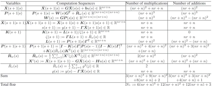
Variables Computation Sequences Number of multiplications Number of additions ˆ X(s+ 1|s) Xˆ(s+ 1|s) =GXˆ(s|s) +bu(s)∈Rnr+n (nr+n)2+nr+n (nr+n)2 P(s+ 1|s) P(s+ 1|s) =W(s)GT+ ˆRw(s)∈R(nr+n)×(nr+n) (nr+n)3 (nr+n)3 W(s) :=GP(s|s)∈R(nr+n)×(nr+n) (nr+n)3 (nr+n)3−(nr+n)2 ˆ X(s+ 1|s+ 1) ˆX(s+ 1|s+ 1) = ˆX(s+ 1|s) +K(s+ 1)s(s+ 1)∈Rnr+n nr+n nr+n s(s+ 1) :=y(s+ 1)−ΓXˆ(s+ 1|s)∈R nr+n nr+n K(s+ 1) K(s+ 1) =L(s+ 1)/ζ(s+ 1)∈Rnr+n nr+n 0 ζ(s+ 1) :=Γ L(s+ 1) + ˆRv(s)∈R nr+n nr+n L(s+ 1) :=P(s+ 1|s)ΓT∈Rnr+n (nr+n)2 (nr+n)2−(nr+n) P(s+ 1|s+ 1) P(s+ 1|s+ 1) = [I−K(s)Γ]P(s|s−1)[I−K(s)Γ]T (nr+n)3+ 4(nr+n)2 (nr+n)3+ 3(nr+n)2 +K(s) ˆRv(s)KT(s)∈R(nr+n)×(nr+n) +(nr+n) ˆ Rw(s) Rˆw(s) =1sPsj=1[X0(j)X0T(j)]∈R(nr+n)×(nr+n) 2(nr+n)2 (nr+n)2 X0(s) := ˆX(s+ 1|s+ 1)−GXˆ(s|s)−Hu(s)∈Rnr+n (nr+n)2+ (nr+n) (nr+n)2+ (nr+n) ˆ Rv(s) Rˆv(s) =s1Psj=1%2(j)∈R 2 1 %(s) :=y(s)−ΓXˆ(s|s)∈R nr+n nr+n Sum 3(nr+n)3+ 9(nr+n)23(nr+n)3+ 3(nr+n)2 +8(nr+n) + 2 +4(nr+n) + 1 Total flop N1:= 6(nr+n)3+ 12(nr+n)2+ 12(nr+n) + 3
The difference of the computation cost between two algorithms at each step is
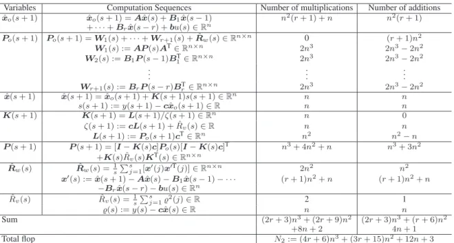
Table II. The computational efficiency of the direct state estimation algorithm based on the delta operator Variables Computation Sequences Number of multiplications Number of additions ˆ xo(s+ 1) xˆo(s+ 1) =Axˆ(s) +B1xˆ(s−1) n2(r+ 1) +n n2(r+ 1) +· · ·+Brxˆ(s−r) +bu(s)∈Rn Po(s+ 1) Po(s+ 1) =W1(s) +· · ·+Wr+1(s) + ˆRw(s)∈Rn×n 0 (r+ 1)n2 W1(s) :=AP(s)AT∈Rn×n 2n3 2n3−2n2 W2(s) :=B1P(s−1)B1T∈Rn×n 2n3 2n3−2n2 .. . ... ... Wr+1(s) :=BrP(s−r)BrT∈Rn×n 2n3 2n3−2n2 ˆ x(s+ 1) xˆ(s+ 1) = ˆxo(s+ 1) +K(s+ 1)s(s+ 1)∈Rn n n s(s+ 1) :=y(s+ 1)−cxˆo(s+ 1)∈R n n K(s+ 1) K(s+ 1) =L(s+ 1)/ζ(s+ 1)∈Rn n 0 ζ(s+ 1) :=cL(s+ 1) + ˆRv(s)∈R n n L(s+ 1) :=Po(s+ 1)cT∈Rn n2 n2−n P(s+ 1) P(s+ 1) = [I−K(s)c]Po(s)[I−K(s)c]T n3+ 4n2+n n3+ 3n2 +K(s) ˆRv(s)KT(s)∈Rn×n ˆ Rw(s) Rˆw(s) = 1sPsj=1[x0(j)x0T(j)]∈Rn×n 2n2 n2 x0(s) := ˆx(s+ 1)−Axˆ(s)−B 1xˆ(s−1)− · · · (r+ 1)n2+n (r+ 1)n2+n −Brxˆ(s−r)−bu(s)∈Rn ˆ Rv(s) Rˆv(s) = s1Psj=1%2(j)∈R 2 1 %(s) :=y(s)−cxˆ(s)∈R n n Sum (2r+ 3)n3+ (2r+ 9)n2 (2r+ 3)n3+ (r+ 6)n2 +8n+ 2 4n+ 1 Total flop N2:= (4r+ 6)n3+ (3r+ 15)n2+ 12n+ 3 −[(4r+ 6)n3+ (3r+ 15)n2+ 12n+ 3] =n3(6r3+ 18r2+ 14r) +n2(12r2 +21r−1) + 12nr.
Assume that the system order n= 10and the delayr= 5, then we can calculate the difference between the computation loads of the two algorithms at each step:
N1−N2= (6×603+ 12×602+ 723) −(26×103+ 30×102+ 123) = 1.3108×10⁶.
Assume that the system order n= 100 and the delay r= 50, then the difference between two algorithms is
N1−N2= (6×51003+ 12×51002+ 12×5100 + 3) −(206×1003+ 165×1002+ 12×100 + 3)
≈8.0×10¹¹.
Table III. The computational comparison between two algorithms
n r N1−N2 (N1−N2)/N1 N2/N1
10 10 8.08×10⁶ 0.993 0.007 20 10 6.41×10⁷ 0.994 0.006 20 20 4.50×10⁸ 0.998 0.002
Remark 7: TablesI–IIIshow the comparison of the computational burden of the two algorithms, which illustrates that the direct state estimation algorithm based on the delta operator can greatly reduce the computational burden compared with the generalized Kalman filtering algorithm, especially for large-scale systems.
4. NUMERICAL EXAMPLES Example 1. Consider a third-order system with time-delay:
x(s+ 1) = · A11 A12 A21 A22 ¸ · x1(s) x2(s) ¸ + · B11 B12 ¸ · x1(s−1) x2(s−1) ¸ + · b1 b2 ¸ u(s) +w(s), y(s) =cx(s) +v(s),
where the parameters are given by
A11= 0.10, A12= [0.40,0.20], A21= · −0.30 −0.20 ¸ , A22= · 0.20 −0.40 0.10 −0.10 ¸ , B11= [0.20,0.60,0.30], B12= · 0.20 −0.20 −0.30 −0.40 −0.20 −0.10 ¸ , b= [0.30,0.50,0.60]T, c= [0.40,0.60,0.50].
In simulation, the input{u(s)} is taken as a persistent excitation signal sequence with zero mean and unit variance, and{v(s)} as a random sequence with the normal distribution, zero mean and varianceRv= 0.102, and{w(s)} as a white noise vector sequence with zero mean and variance
Rw= 0.052I3. Take the data lengthL= 300as the data length, and apply the direct state estimation
algorithm in (30)–(36) to estimate the states of the considered system. The system input u(s), the true output y(s) and the predicted output yˆ(s) are shown in Figure 1. The states x(s) and their estimatesxˆ(s)and errors versus sby the generalized Kalman filtering algorithm are shown in Figures 2–4. The states x(s)and their estimates xˆ(s) and errors versus s by the direct state estimation algorithm are shown in Figures5–7. The root mean squares error is used to describe the error between the true statexi(s)and its estimated valueˆxi(s), and the error between the true output
y(s)and its predicted outputyˆ(s), which are defined as
Errorx= ( 1 L L X s=1 [ˆxi(s)−xi(s)]2 )1/2 , Errory= ( 1 L L X s=1 [ˆy(s)−y(s)]2 )1/2 .
The results are shown in TablesIVandV.
Table IV. The root mean squares error of the generalized Kalman filtering algorithm
Rv Rw x1(s) x2(s) x3(s) y(s)
0.102 0.052I6 0.22360 0.21388 0.24850 0.21475
0.052 0.102I6 0.28187 0.27252 0.27762 0.22835
Example 2. Consider the following system:
x(s+ 1) = AA1121 AA1222 AA1323 A31 A32 A33 xx12((ss)) x3(s) + BB1112 B13 xx12((ss−−1)1) x3(s−1) + bb12 b3 u(s) +w(s),
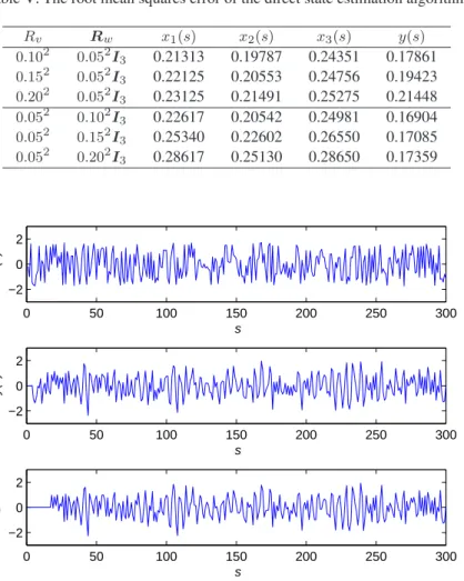
Table V. The root mean squares error of the direct state estimation algorithm Rv Rw x1(s) x2(s) x3(s) y(s) 0.102 0.052I3 0.21313 0.19787 0.24351 0.17861 0.152 0.052I3 0.22125 0.20553 0.24756 0.19423 0.202 0.052I3 0.23125 0.21491 0.25275 0.21448 0.052 0.102I3 0.22617 0.20542 0.24981 0.16904 0.052 0.152I3 0.25340 0.22602 0.26550 0.17085 0.052 0.202I3 0.28617 0.25130 0.28650 0.17359 0 50 100 150 200 250 300 −2 0 2 s u(s) 0 50 100 150 200 250 300 −2 0 2 s y(s) 0 50 100 150 200 250 300 −2 0 2 s y 1 (s)
Figure 1. The system inputu(s), outputy(s)and the predicted outputyˆ(s)versuss
0 50 100 150 200 250 300 −3 −2 −1 0 1 2 3 s State estimate of x 1 (s) x1(s) ˆ x1(s) ˆ x1(t)−x1(s)
Figure 2. Statex1(s)and the estimated statexˆ1(s)versussby the generalized Kalman filtering algorithm
y(s) =cx(s) +v(s),
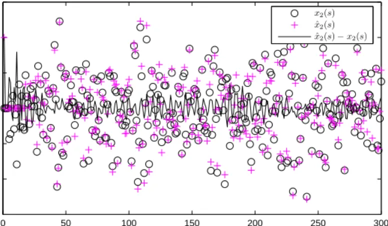
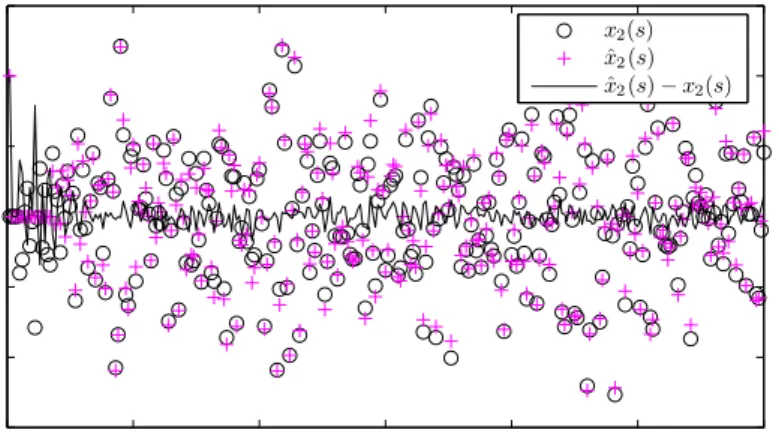
0 50 100 150 200 250 300 −3 −2 −1 0 1 2 3 s State estimate of x 2 (s) x2(s) ˆ x2(s) ˆ x2(s)−x2(s)
Figure 3. Statex2(s)and the estimated statexˆ2(s)versussby the generalized Kalman filtering algorithm
0 50 100 150 200 250 300 −3 −2 −1 0 1 2 3 s State estimate of x 3 (s) x3(s) ˆ x3(s) ˆ x3(s)−x3(s)
Figure 4. Statex3(s)and the estimated statexˆ3(s)versussby the generalized Kalman filtering algorithm
0 50 100 150 200 250 300 −3 −2 −1 0 1 2 3 s State estimate of x 1 (s) x1(s) ˆ x1(s) ˆ x1(s)−x1(s)
0 50 100 150 200 250 300 −3 −2 −1 0 1 2 3 s State estimate of x 2 (s) x 2(s) ˆ x 2(s) ˆ x 2(s)−x2(s)
Figure 6. Statex2(s)and the estimated statexˆ2(s)versussby the direct state estimation algorithm
0 50 100 150 200 250 300 −3 −2 −1 0 1 2 3 s State estimate of x 3 (s) x 3(s) ˆ x 3(s) ˆ x 3(s)−x3(s)
Figure 7. Statex3(s)and the estimated statexˆ3(s)versussby the direct state estimation algorithm
where the parameters are given by
A11= 0.10, A12= [0.20,−0.20],A13= [0.50,−0.30,0.20], A21= · −0.30 0.20 ¸ , A22= · 0.20 −0.22 0.30 −0.10 ¸ ,A23= · 0.25 0.15 −0.25 0.30 −0.15 0.40 ¸ , A31= −00.14.15 −0.25 , A32= −00.12 00..2522 −0.20 0.30 , A33= 0.025 00..3020 −−00..2130 −0.20 0.35 0.15 , B11= [0.20,0.40,0,0.10,0.30,−0.25], B12= · 0.32 0.12 −0.25 0.25 0.30 0.20 −0.35 0.15 −0.15 0.25 0 0.25 ¸ , B13= −00.20.14 −00.30.22 0.015 −00.26.25 00..1043 −00.25.15 −0.20 −0.30 −0.45 0.15 0.45 0.25 ,
b1= 0.3, b2= [0.5,0.6]T, b3= [0.35,0.40,0.60]T, c= [0.4,0.6,0.5,0.3,0.2,0.1].
The simulation condition is the same as that in Example 1. Take {v(s)} as a random sequence with the normal distribution, zero mean and variance Rv= 0.102, and {w(s)} as a white noise
vector sequence with zero mean and varianceRw= 0.052I6. Take the data lengthL= 300as the
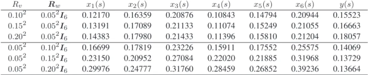
data length, and apply the direct state estimation algorithm in (30)–(36) to estimate the states of the considered system. The system inputu(s), the true outputy(s)and the predicted outputyˆ(s) are shown in Figure8. The statex(s)and their estimates xˆ(s)and errors versuss are shown in Figures9–11and TableVI.
Table VI. The root mean squares error of the algorithm
Rv Rw x1(s) x2(s) x3(s) x4(s) x5(s) x6(s) y(s) 0.102 0.052I6 0.12170 0.16359 0.20876 0.10843 0.14794 0.20944 0.15523 0.152 0.052I6 0.13191 0.17089 0.21133 0.11074 0.15249 0.21055 0.16663 0.202 0.052I6 0.14383 0.17980 0.21433 0.11396 0.15810 0.21204 0.18057 0.052 0.102I6 0.16699 0.17819 0.23226 0.15911 0.17552 0.25575 0.14069 0.052 0.152I6 0.23150 0.20952 0.27084 0.22020 0.21885 0.31968 0.13729 0.052 0.202I6 0.29976 0.24777 0.31760 0.28459 0.26852 0.39236 0.13664 0 50 100 150 200 250 300 −2 0 2 s u(s) 0 50 100 150 200 250 300 −4 −2 0 2 4 s y(s) 0 50 100 150 200 250 300 −4 −2 0 2 4 s y 1 (s)
Figure 8. The system inputu(s), outputy(s)and the predicted outputyˆ(s)versuss
From the simulation results in Tables I–V and Figures 1–11, we can draw the following conclusions.
• The state estimation accuracy of the direct state estimation algorithm is approximate to that of the generalized Kalman filtering algorithm. They both has good performance because the estimated states are close to their true values withs increasing. However, the direct state estimation algorithm requires less computational cost compared with the generalized Kalman filtering algorithm, see TablesI–V, and Figures2–7and Figures9–11.
0 50 100 150 200 250 300 −2 −1 0 1 2 s State estimate of x 1 (s) 0 50 100 150 200 250 300 −2 −1 0 1 2 s State estimate of x 2 (s)
Figure 9. Statesx1(s),x2(s)and the estimated statesxˆ1(s)andxˆ2(s)versuss
0 50 100 150 200 250 300 −2 −1 0 1 2 3 s State estimate of x 3 (s) 0 50 100 150 200 250 300 −1 0 1 2 s State estimate of x 4 (s)
Figure 10. Statesx3(s),x4(s)and the estimated statesxˆ3(s)andxˆ4(s)versuss
• The proposed estimation algorithm can generate good estimates because the predicted output is close to the true output, see TablesV–VI, and Figures1and8.
• The state estimation accuracy of the proposed algorithm becomes better under the lower noise levels, see TablesV–VI.
0 50 100 150 200 250 300 −2 −1 0 1 2 s State estimate of x 5 (s) 0 50 100 150 200 250 300 −3 −2 −1 0 1 2 3 s State estimate of x 6 (s)
Figure 11. Statesx5(s),x6(s)and the estimated statesxˆ5(s)andxˆ6(s)versuss
5. CONCLUSIONS
This paper studies the state estimation for linear systems with multi-state-delays from observation data. A state estimation algorithm based on the Kalman filtering principle is proposed for comparison. A direct state estimation algorithm is presented by minimizing the state estimation error covariance matrix based on the delta operator. The computational complexity analysis shows that the direct state estimation algorithm requires less computational cost than the generalized state estimation algorithm. The simulation results show that the direct state estimation algorithm can generate accurate estimates. The methods proposed in this paper can combine some statistical methods [48-55] to studu the parameter identification and state filter design for different systems with coloured noise [56-62].
ACKNOWLEDGEMENT
This work was supported by the National Natural Science Foundation of China under grant number 61873111, and the 111 Project (B12018) and the Postgraduate Research and Practice Innovation Program of Jiangsu Province under grant number KYCX18−1854.
REFERENCES
1. Svensson A, Sch¨on TB. A flexible state-space model for learning nonlinear dynamical systems. Automatica. 2017;80:189-199.
2. Xu L, Ding F, Zhu,QM. Hierarchical Newton and least squares iterative estimation algorithm for dynamic systems by transfer functions based on the impulse responses.International Journal of Systems Science. 2019;50(1):141-151.
3. Xu L, Ding F. Parameter estimation algorithms for dynamical response signals based on the multi-innovation theory and the hierarchical principle.IET Signal Processing. 2017;11(2):228-237.
4. Xu L. Application of the Newton iteration algorithm to the parameter estimation for dynamical systems.Journal of Computational and Applied Mathematics. 2015;288:33-43.
5. Pan J, Ma H, Jiang X, et al. Adaptive gradient-based iterative algorithm for multivariate controlled autoregressive moving average systems using the data filtering technique.Complexity. 2018. Article ID 9598307. https://doi.org/10.1155/2018/9598307
6. Wan XK, Wu H, Qiao F, et al. Electrocardiogram baseline wander suppression based on the combination of morphological and wavelet transformation based filtering.Computational and Mathematical Methods in Medicine. 2019. Article ID 7196156. https://doi.org/10.1155/2019/7196156
7. Chen J, Liu Y, Xu L. A new filter-based stochastic gradient algorithm for dual-rate ARX models.International Journal of Adaptive Control and Signal Processing. 2018;32(11):1557-1568.
8. Wang YJ, Ding F. A filtering based multi-innovation gradient estimation algorithm and performance analysis for nonlinear dynamical systems.IMA Journal of Applied Mathematics. 2017;82(6):1171-1191.
9. Xu L, Ding F, Gu Y, Alsaedi A, Hayat T. A multi-innovation state and parameter estimation algorithm for a state space system with d-step state-delay.Signal Processing. 2017;140:97-103.
10. Sch¨on T, Wills A, Ninness B. System identification of noninear state-space models.Automatica. 2011;47(1):39-49.
11. Partovibakhsh M, Liu G. An adaptive unscented Kalman filtering approach for online estimation of model parameters and state-of-charge of lithium-ion batteries for autonomous mobile robots. IEEE Transactions on Control Systems Technology. 2015;23(1):357-363.
12. Xu L, Xiong WL, A. Alsaedi A, Hayat T. Hierarchical parameter estimation for the frequency response based on the dynamical window data.International Journal of Control Automation and Systems. 2018;16(4):1756-1764.
13. Xu L, Ding F. Iterative parameter estimation for signal models based on measured data.Circuits Systems and Signal Processing. 2018;37(7):3046-3069.
14. Xu L, Ding F. Recursive least squares and multi-innovation stochastic gradient parameter estimation methods for signal modeling.Circuits Systems and Signal Processing. 2017;36(4):1735-1753.
15. Liu SY, Ding F, Xu L, Hayat T. Hierarchical principle-based iterative parameter estimation algorithm for dual-frequency signals.Circuits Systems and Signal Processing. 2019;38. https://doi.org/10.1007/s00034-018-1015-1
16. Xu L. The parameter estimation algorithms based on the dynamical response measurement data.Advances in Mechanical Engineering. 2017;9(11):1-12. doi: 10.1177/1687814017730003
17. Xu L. The damping iterative parameter identification method for dynamical systems based on the sine signal measurement.Signal Processing. 2016;120:660-667.
18. Xu L, Ding F. Parameter estimation for control systems based on impulse responses.International Journal of Control Automation and Systems. 2017;15(6):2471-2479.
19. Xu L, Chen L, Xiong WL. Parameter estimation and controller design for dynamic systems from the step responses based on the Newton iteration.Nonlinear Dynamics. 2015;79(3):2155-2163.
20. Chen J, Huang B, Ding F, Gu Y. Variational Bayesian approach for ARX systems with missing observations and varying time-delays.Automatica. 2018;94:194-204.
21. Gu Y, Chou Y, Liu J, Ji Y. Moving horizon estimation for multirate systems with time-varying time-delays.Journal of the Franklin Institute. 2019;356(4):2325-2345.
22. Pan J, Li W, Zhang HP. Control algorithms of magnetic suspension systems based on the improved double exponential reaching law of sliding mode control.International Journal of Control Automation and Systems. 2018;16(6):2878-2887.
23. Chen J, Zhu QM, Li J, Liu YJ. Biased compensation recursive least squares-based threshold algorithm for time-delay rational models via redundant rule.Nonlinear Dynamics. 2018;91(2):797-807.
24. Shi P, Zhang Y, Agarwal RK. Stochastic finite-time state estimation for discrete time-delay neural networks with Markovian jumps.Neurocomputing. 2015;151:168-174.
25. Xu L. A proportional differential control method for a time-delay system using the Taylor expansion approximation. Applied Mathematics and Computation. 2014;236:391-399.
26. Gu Y, Ding F, Li JH. States based iterative parameter estimation for a state space model with multi-state delays using decomposition.Signal Processing. 2015;106:294-300.
27. Chen GY, Gan M, Chen CP, Li HX. A regularized variable projection algorithm for separable nonlinear least-squares problems.IEEE Transactions on Automatic Control. 2019;64(2):526-537.
28. Chen GY, Gan M, Ding F, Chen CP. Modified Gram-Schmidt method-based variable projection algorithm for separable nonlinear models. IEEE Transactions on Neural Networks and Learning Systems. (2019). doi: 10.1109/TNNLS.2018.2884909
29. Gan M, Chen CPL, Chen GY, Chen L. On some separated algorithms for separable nonlinear least squares problems. IEEE Transactions on Cybernetics. 2018;48(10):2866-2874.
30. Gan M, Li HX. An efficient variable projection formulation for separable nonlinear least squares problems.IEEE Transactions on Cybernetics. 2014;44(5):707-711.
31. Gan M, Li HX, Peng H. A variable projection approach for efficient estimation of RBF-ARX model. IEEE Transactions on Cybernetics. 2015;45(3):462-471.
32. Gan M, Chen CLP, Li HX, Chen L. Gradient radial basis function based varying-coefficient autoregressive model for nonlinear and nonstationary time series.IEEE Signal Processing Letters. 2015;22(7):809-812.
33. Gan M, Chen CLP, Chen L, Zhang CY. Exploiting the interpretability and forecasting ability of the RBF-AR model for nonlinear time series.International Journal of Systems Science. 2016;47(8):1868-1876.
34. Cao Y, Lu H, Wen T. A safety computer system based on multi-sensor data processing.Sensors. 2019;19(4). https://doi.org/10.3390/s19040818
35. Cao Y, Zhang Y, Wen T, Li P. Research on dynamic nonlinear input prediction of fault diagnosis based on fractional differential operator equation in high-speed train control system.Chaos. 2019;29(1). Article Number: 013130. https://doi.org/10.1063/1.5085397
36. Cao Y, Li P, Zhang Y. Parallel processing algorithm for railway signal fault diagnosis data based on cloud computing.Future Generation Computer Systems. 2018;88:279-283.
37. Cao Y, Ma LC, Xiao S, et al. Standard analysis for transfer delay in CTCS-3.Chinese Journal of Electronics. 2017;26(5):1057-1063.
38. Cao Y, Wen Y, Meng X, Xu W. Performance evaluation with improved receiver design for asynchronous coordinated multipoint transmissions.Chinese Journal of Electronics. 2016;25(2):372-378.
39. Zhang YZ, Cao Y, Wen YH, Liang L, Zou F. Optimization of information interaction protocols in cooperative vehicle-infrastructure systems.Chinese Journal of Electronics. 2018;27(2):439-444.
40. Zhang X, Xu L, Ding F, et al. Combined state and parameter estimation for a bilinear state space system with moving average noise.Journal of the Franklin Institute. 2018;355(6):3079-3103.
41. Zhang X, Ding F, Alsaadi FE, Hayat T. Recursive parameter identification of the dynamical models for bilinear state space systems.Nonlinear Dynamics. 2017;89(4): 2415-2429.
42. Zhang X, Ding F, Xu L, Yang EF. State filtering-based least squares parameter estimation for bilinear systems using the hierarchical identification principle.IET Control Theory Applications. 2018;12(12):1704-1713.
43. Zhao SY, Shmaliy YS, Ahn CK, Liu F. Adaptive-horizon iterative UFIR filtering algorithm with applications.IEEE Transactions on Industrial Electronics. 2018;65(8):6393-6402.
44. Shi Y, Fang H, Yan M. Kalman filter-based adaptive control for networked systems with unknown parameters and randomly missing outputs.International Journal of Robust and Nonlinear Control. 2009;19(18):1976-1992.
45. Kim JH. Note on stability of linear systems with time-varying delay.Automatica. 2011;47(9):2118-2121.
46. Liu H, Lu JA, L¨u J, Hill DJ. Structure identification of uncertain general complex dynamical networks with time delay.Automatica. 2009;45(8):1799-1807.
47. Golub GH, Van Loan CF.Matrix Computations. Baltimore, MD: Johns Hopkins University Press; 1996.
48. Yin CC, Zhao JS. Nonexponential asymptotics for the solutions of renewal equations, with applications.Journal of Applied Probability. 2008;43(3):815-824.
49. Gao HL, Yin CC. The perturbed sparre Andersen model with a threshold dividend strategy. Journal of Computational and Applied Mathematics. 2008;220(1-2):394-408.
50. Yin CC, Yuen KC. Optimality of the threshold dividend strategy for the compound Poisson model.Statistics & Probability Letters. 2011;81(12):1841-1846.
51. Yin CC, Wen YZ. Exit problems for jump processes with applications to dividend problems. Journal of Computational and Applied Mathematics. 2013;245:30-52.
52. Yin CC, Wen YZ. Optimal dividend problem with a terminal value for spectrally positive Levy processes.Insurance Mathematics & Economics. 2013;53(3):769-773.
53. Yin CC, Wang CW. The perturbed compound Poisson risk process with investment and debit interest.Methodology and Computing in Applied Probability. 2010;12(3):391-413.
54. Yin CC, Wen YZ, Zhao YX. On the optimal dividend problem for a spectrally positive levy process.Astin Bulletin. 2014;44(3):635-651.
55. Yin CC, Zhao JS. Nonexponential asymptotics for the solutions of renewal equations with applications.Journal of Applied Probability. 2006;43(3):815-824.
56. Hu YB, Zhou Q, Yu H, Zhou Z, Ding F. Two-stage generalized projection identification algorithms for controlled autoregressive systems.Circuits Systems and Signal Processing. 2019;38. https://doi.org/10.1007/s00034-018-0996-0
57. Ge ZW, Ding F, Xu L, Alsaedi A, Hayat T. Gradient-based iterative identification method for multivariate equation-error autoregressive moving average systems using the decomposition technique.Journal of the Franklin Institute. 2019;356(3):1658-1676.
58. Wan LJ, Ding F. Decomposition- and gradient-based iterative identification algorithms for multivari-able systems using the multi-innovation theory. Circuits Systems and Signal Processing. 2019;38. https://doi.org/10.1007/s00034-018-1014-2
59. Liu QY, Ding F. Auxiliary model-based recursive generalized least squares algorithm for multivariate output-error autoregressive systems using the data filtering.Circuits Systems and Signal Processing. 2019;38(2):590-610.
60. Ding JL. The hierarchical iterative identification algorithm for multi-input-output-error systems with autoregressive noise.Complexity. 2017;1-11. Article ID 5292894. https://doi.org/10.1155/2017/5292894
61. Xu H, Ding F, Yang EF. Modeling a nonlinear process using the exponential autoregressive time series model. Nonlinear Dynamics. 2019. https://doi.org/10.1007/s11071-018-4677-0
62. Ding F, Liu XP, Liu G. Gradient based and least-squares based iterative identification methods for OE and OEMA systems.Digital Signal Processing. 2010;20(3):664-677.