HAL Id: hal-02355503
https://hal.archives-ouvertes.fr/hal-02355503
Submitted on 8 Nov 2019
HAL
is a multi-disciplinary open access
archive for the deposit and dissemination of
sci-entific research documents, whether they are
pub-lished or not. The documents may come from
teaching and research institutions in France or
abroad, or from public or private research centers.
L’archive ouverte pluridisciplinaire
HAL
, est
destinée au dépôt et à la diffusion de documents
scientifiques de niveau recherche, publiés ou non,
émanant des établissements d’enseignement et de
recherche français ou étrangers, des laboratoires
publics ou privés.
FSSD - A Fast and Efficient Algorithm for Subgroup Set
Discovery
Adnene Belfodil, Aimene Belfodil, Anes Bendimerad, Philippe Lamarre,
Céline Robardet, Mehdi Kaytoue, Marc Plantevit
To cite this version:
Adnene Belfodil, Aimene Belfodil, Anes Bendimerad, Philippe Lamarre, Céline Robardet, et al.. FSSD
- A Fast and Efficient Algorithm for Subgroup Set Discovery. IEEE International Conference on Data
Science and Advanced Analytics (DSAA), Oct 2019, Washington DC, United States. �hal-02355503�
FSSD - A Fast and Efficient Algorithm for
Subgroup Set Discovery
Adnene Belfodil
*,1, Aimene Belfodil
*,1,2, Anes Bendimerad
1,
Philippe Lamarre
1, C´eline Robardet
1, Mehdi Kaytoue
1,3, Marc Plantevit
41
Univ Lyon, INSA Lyon, CNRS, LIRIS UMR 5205, F-69621, LYON, France
2
Mobile Devices Ingeni´erie, 100 Avenue Stalingrad, 94800, Villejuif, France
3Infologic, 99 avenue de Lyon, 26500 Bourg-L`es-Valence, France
4
Univ Lyon, CNRS, LIRIS UMR 5205, F-69621, LYON, France
[email protected]
Abstract—Subgroup discovery (SD) is the task of discovering interpretable patterns in the data that stand out w.r.t. some prop-erty of interest. Discovering patterns that accurately discriminate a class from the others is one of the most common SD tasks. Standard approaches of the literature are based on local pattern discovery, which is known to provide an overwhelmingly large number of redundant patterns. To solve this issue, pattern set mining has been proposed: instead of evaluating the quality of patterns separately, one should consider the quality of a pattern set as a whole. The goal is to provide a small pattern set that is diverse and well-discriminant to the target class. In this work, we introduce a novel formulation of the task of diverse subgroup set discovery where both discriminative power and diversity of the subgroup set are incorporated in the same quality measure. We propose an efficient and parameter-free algorithm dubbedFSSD and based on a greedy scheme. FSSD uses several optimization strategies that enable to efficiently provide a high quality pattern set in a short amount of time.
Index Terms—Pattern Mining, Subgroup Discovery. I. INTRODUCTION
Data science can be seen as a language that allows, among others, the analysis of (large amount of) data [43]. Following the same philosophy of Exploratory Data Analysis (EDA) [47], one of the main tasks of data science is the discovery of interpretable and understandable patterns in the data, a task known as data mining [11]. Subgroup discovery (SD) [27], [50] is a popular data mining task that aims, amongst many other possibilities, to discover patterns describing regions in a dataset where the distribution of the target variable signif-icantly deviates from the norm. For instance, a subgroup de-fined by the description age≥ 65∧smoker =true fosters the target variable “lung cancer” prevalence in some patient-dataset.
In SD, as in most of local pattern mining approaches, an important problem that one has to consider is the huge number of patterns (subgroups) that can be produced. Many of these subgroups are redundant and convey very similar information. This issue notably becomes more serious when the number and/or the domain of attributes is large. This challenge led
* Both authors contributed equally to this work.
to the definition of the pattern set mining problem [8], [20], [28], [40]. Whilelocal pattern miningseeks for patterns where each of them satisfies local constraints individually, pattern set mining aims to find a small set of patterns that together satisfy global constraints. These global constraints are used to guarantee the diversity in the returned pattern set. Different approaches exist in the literature to tackle the problem of pattern set mining:
(1) Non-diversified top-k approach.Such algorithms output the top-k best subgroups (e.g., BSD [32] and MiSoSouP
[41]). Although this allows to control the number of returned patterns, this does not solve the redundancy problem since the top-k patterns can be very similar and describe only a few of all the local optima (lack of diversity).
(2) Exhaustive approach.Such methods aim to find the best possible solution. The pioneering work of [40] proposes a level wise algorithm to explore the search space, and [21], [26], [38] use a Constraint Programming (CP) solver to retrieve the k-pattern set. In large and complex datasets, the exhaustive selection of the best k-pattern set becomes unfeasible, even if pruning strategies are used. As the number of possible pattern sets is exponential in the size of the set of local patterns, which is itself huge, the computational efficiency of pattern set mining is a very challenging task. In fact, the general problem of pattern set discovery is NP-hard [35].
(3) Two-step approach. These algorithms start by (a) gen-erating a collection of local patterns by some exhaustive or heuristic technique followed by (b) a heuristic selection of a smaller subset of complementary patterns [5], [8], [44]. However, since the number of local patterns can be large, these algorithms need a huge amount of memory to store them. Moreover, post-processing the set of all mined local patterns can be time-consuming. Noteworthy algorithms belonging to this family are: DSSD[48] andMCTS4DM[7].
(4) Sequential covering approach. Algorithms proposed in [9], [31], [46] use the so-called sequential coveringstrategy for subgroup set discovery. These algorithms repeatedly and heuristically (i.e. beam search) look for one subgroup; add it to the already constituted subgroup set; then re-weight or
delete the already covered objects in the database in the aim of reducing their impact in the next iterations. This approach allows to implicitly consider the diversity of the produced subgroup set, conversely to some two-step approaches where an additional “diversity” measure is used.
Contributions. In this paper, we investigate the problem of
subgroup set discovery, i.e. “discovery of a non-redundant set of high-quality subgroups.” [48]. This can be seen as a particular instance of the more general task of pattern set mining. After formally introducing the notion of SD-compatible quality measures (e.g. WRAcc) that locally eval-uate subgroups interestingness, we extend their definitions to subgroup sets. This allows to evaluate the interestingness of a subgroup set in terms of its discriminative power and diversity. We propose a greedy scheme to maximize these measures by incrementally augmenting the subgroup set with subgroups providing the highest marginal contribution. In this respect, we devise a branch-and-bound algorithm, dubbed FSSD, a
parameter-free and memory efficient algorithm tailored for diverse subgroup set discovery. It exploits (i) tight optimistic estimates on the marginal contributions of SD-compatible measures to prune unpromising branches, (ii) closure operators to efficiently explore the search space and (iii) successive removal of already covered objects (i.e. sequential covering) to significantly reduce candidate subgroups.
Outline.The remainder of this paper is organised as follows. Sec. II recalls preliminary notions. Sec. III introduces the problem ofk-diverse subgroup set discovery. Sec. IV presents the generic greedy framework. Sec. V introducesFSSD. While the approximation ratio to the best possible solution of the proposed problem is not theoretically bounded, Sec. VI reports a thorough empirical study that demonstratesFSSDefficiency and effectiveness. Sec. VII concludes the paper.
II. PRELIMINARIES
In this paper, for any setE,℘(E)denotes the powerset of
E. Forf :E→F and a subsetA⊆E, the image ofAbyf
is denoted by f[A] (i.e. f[A] ={f(a)|a∈A}). Details on order-theoretic notions can be found in [42].
A. Input dataset.
A dataset is a pair(G,A) whereG is a set of objects and
A={ai}1≤i≤mis an ordered set of attributes. Each attribute
a ∈ A can be seen as a mapping a: G → Ra whereRa is
called the domain of the attribute. For instance, Ra is given
by R if a is numerical, by a finite set of categories Ci if a
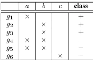
is nominal (categorical) or by {0,1} if a is Boolean. Each objectg∈ G is labeled as eitherpositiveornegative. It means that G is partitioned into two subsets G+ and G− enclosing
respectively positive and negative instances. The proportion
α:= |G+|/|G| is called the positive prevalence. Fig. 1 (left)
depicts a dataset containing 3 attributes of distinct types where
G+ = {g
2, g3, g5} is the set of individuals having a high
income.
B. Pattern Language
Apatterndis aconstrained selectorof a subset of objects of the dataset using their attribute values. We refer to the set of all possible patterns that we want to explore by thepattern language and we denote it D. In our case, D =
×
mi=1Diwhere Di is given by the set of all possible intervals in R
if ai is numerical, the set {Ci,∅} ∪ {{c} | c ∈ Ci} if ai is
nominal or{{0,1},{1}}ifaiis Boolean (i.e. if negative item
{0}needs to be considered, attributeaineeds to be considered
as nominal). A pattern d ∈ D is then given by a sequence of restrictions over each attribute (i.e. d = (di)1≤i≤m). For
example, in Fig. 1 (right) pattern d = ({0,1},{M},R) is read “individual that are married or not, men and having any age”. Note that we considered here the exhaustive search space for the numerical attributes as in [7], [25] and noapriori
discretization is performed.
As when we deal with itemsets, patterns in D are or-dered from the most general one to the most restrictive one by an order relation v. In our case, for two patterns
c = (ci)1≤i≤m ∈ D and d = (di)1≤i≤m ∈ D, we have:
c v d ⇔ ∀i ∈ J1, mK(ci ⊇ di). In Fig. 1 (right), pattern
c = ({0,1},{M},R) is less restrictive than pattern d =
({0,1},{M},[27,65]) (i.e. c v d) since d has an additional constraint on the age attribute. One can show that the partially ordered set(D,v)is a meet-semilattice (the meet is denoted
u). It means that for allc, d∈ D, there is maximum common lower boundcud(i.e.(∀e∈ D)evc∧evd⇔evcud). Given the pattern language explained above, we should link objects in G to descriptions in D. This is done by the cover
relationship. A description d ∈ D is said to cover g ∈ G
iff ∀i ∈ J1, mK : ai(g) ∈ di. Each object g ∈ G is now
mapped to the most-restrictive descriptionδ(g)∈ D covering it: ∀d ∈ D, d covers g iff d v δ(g). Fig. 1 illustrates this mappings between objects and descriptions.
C. Pattern Structure
Pattern structure is a generalization of the Formal Concept Analysis (FCA) framework [13] to complex attributes such as numerical and nominal ones (see [14] for further details). Since(D,v)is a meet-semilattice, the triple(G,(D,v), δ)is pattern structure. This triple contains all information we need to search for patterns in a dataset and allows us to use an algorithm like Close-by-One (CbO) [29] to exhaustively enu-merate them. Two mappings associated to a pattern structure are important to keep in mind: (1) ext : D → ℘(G), d 7→ {g ∈ G | d v δ(g)} called the extent. It associates to each pattern d ∈ D the set of objects in G for which d hold. (2) int : ℘(G) → D, E 7→ d
g∈Eδ(g) associates to each
subset E ⊆ G the most-restrictive pattern d ∈ D covering them. Note that ext is order-reversing: i.e. if c v d then
ext(d) ⊆ ext(c) (i.e. if d is more restrictive than c, then
d covers less objects than c), property from which (anti)-monotonicity of some measures ensues. Note also thatint◦ext
and ext◦intare closure operators since the pair (ext, int)
married? sex age income g1 × I 23 ≤50k g2 × M 27 >50k g3 M 65 >50k g4 F 54 ≤50k g5 × F 43 >50k g6 M 13 ≤50k mappingδ income g1 ({1},{I},[23,23]) ≤50k g2 ({1},{M},[27,27]) >50k g3 ({0,1},{M},[65,65]) >50k g4 ({0,1},{F},[54,54]) ≤50k g5 ({1},{F},[43,43]) >50k g6 ({0,1},{M},[13,13]) ≤50k
Descriptions and their extents:
c= ({0,1},{M},R), ext(c) ={g2, g3, g6}
d= ({0,1},{M},[27,65]), ext(d) ={g2, g3}
Fig. 1: A labeled dataset(left), objects and their descriptions(center)and some descriptions inD(right)
III. PROBLEMDEFINITION
A. Subgroups and their interestingness.
A subgroup s is any subset of objects in S = ext[D] =
{ext(d)|d∈ D}. We choose to describe subgroups by their
intents since they provide the most specific (most insightful) description. For instance, in Figure 1, the set {g2, g3} is a
subgroup whose intent is d= ({0,1},{M},[27,65]). Indeed, any refinement of the description d will drop at least one object.
A measureφ:℘(G)×℘(G)→R; (s, U)7→φ(s, U)defines
a mapping that evaluates some property of a subgroup s ∈ ℘(G) in the sub-dataset U ⊆ G. For the sake of clarity, if the second parameter U is omitted, then U is the whole set of objects G. The very basic measure is the relative support :
relsup:s, U7→ |s∩U|/|U|.
The relative support is monotonic w.r.t. parameter1(i.e.s⊆ t⇒relsup(s, U)≤relsup(t, U)). Using the relative support, thetrue positive rate(tpr)and thefalse positive rate(f pr)of a subgroup sare defined respectively as follows tpr(s, U) = relsup(s,G+∩U)andf pr(s, U) =relsup(s,G−∩U). Every
objective measure ([17]) can be written using tpr, f pr and some constants. Properties of measures w.r.t. the task have been thoroughly studied in the literature [12], [24], [33], [39]. For a SD task, we define SD-compatiblemeasures.
Definition 1. A measure φ is said to be SD-compatible if the following property ∀s1, s2 ∈S: iftpr(s1)≥tpr(s2)and
f pr(s1)≤f pr(s2)thenφ(s1)≥φ(s2). In other words, ifs1
dominates s2 in the ROC space (i.e.tpr-vs.-f pr space), then
φ(s1)≥φ(s2).
Almost all usual measures in SD are SD-compatibles. For instance, Weighted Relative Accuracy (WRAcc), Accuracy, correlation coefficient, Cohen’s kappa, m-estimate, G-measure and Fβ-measure among others are SD-compatible (see
Ap-pendix C). Please note that, preferably, other properties must hold for a measure in order to be usefulfor a SD task (e.g. constant in independence case, i.e. tpr=f pr [33]).
B. Subgroup Sets Interestingness.
A subgroup set is a set S ⊆ S. Following [40], subgroup
sets are interpreted asdisjunctions of subgroups. Accordingly, the set of objects covered by a subgroup set is given by the union of its subgroups. To evaluate the interestingness of a
subgroup set S , we extend the quality measure φ definition as followsφ(S) =φ S
s∈Ss
since the description associated to S is the disjunction of the intent of each subgroup. Such a formulation gives higher quality φ(S) to subgroups in S
covering different regions.
C. Problem - Subgroup Set Discovery.
Problem Statement. Let be a dataset (G,A), a cardinality constraintk∈Nand a SD-compatible measureφ. Output one subgroup set fromargmaxS⊆S,|S|≤kφ(S).
To the best of the authors’ knowledge, this is a novel way to present the problem of diverse subgroup set discovery. It has the advantage that both discriminative power and diversity of the subgroup set are incorporated into the same measure. It is worth to note that Problem III-C, even when Sis considered
as an input, is NP-Hard. For the convenience of the reader, we delay the proof to Appendix A. One naive (exact) solution for this problem is: (1) look for all possible subgroups in the first phase then (2) test all possible sets of subgroups which size is belowk. However, such a solution is practically unfeasible.
IV. A GREEDYSOLUTION
To approximate the exact solution of problem III-C, we rely on a greedy optimization algorithm. Before presenting such a solution, we present below in Definition 2 the notion of marginal contribution associated to some quality measure.
Definition 2. For a measureφand a subgroup setS ⊆S, the
marginal contributiontoS is the functionφS:
φS :℘(G)→R;s7→φ
[
S ∪s−φ[S
The marginal contributionφS quantifies the qualityφgain that
a subgroup sbrings to the subgroup set S if added.
A. The Greedy Scheme.
Algorithm 1 presents the general scheme of a greedy solution [36]. It starts by an empty subgroup set (line 1). Next, it incrementally constitutes the subgroup setSby successively adding the subgroup s∗ providing the top marginal
contribu-tion (line 3). Algorithm 1 stops when |S|=k or there is no subgroup providing a positive marginal contribution.
When studying the quality of a greedy approach solution, one need to evaluate the so-calledapproximation ratio. How-ever, since quality measures φ : ℘(S) → R extended to
Algorithm 1: Greedy solution for Problem III-C
Input:(G,A)labeled dataset,k∈N, a measureφ
1 S ← {}
2 while|S|< kdo
3 Look fors∗∈argmaxs∈SφS(s)
4 ifφS(s∗)>0 then S ← S ∪ {s∗} else Break 5 returnS
a b c class g1 × + g2 × + g3 × + g4 × × − g5 × × − g6 × −
TABLE I: Dataset with boolean descriptive attributes
subgroup sets are not necessarily sub-modular [36], one cannot use the usual lower bound on the approximation ratio, i.e.
1−1 e.
Definition 3. Let φ be a measure, k be the cardinality constraint and Sgreedy be the output of Algorithm 1 w.r.t.k.
The approximation ratio ρof Sgreedy is given by:
ρ(Sgreedy) =
φ(Sgreedy)
maxS∈S,|S|≤kφ(S)
N.B. maxS∈S,|S|≤kφ(S) = 0⇒ρ(Sgreedy) = 1.
Unfortunately, the quality of the greedy solution cannot be theoretically guaranteed (i.e. lower-bounded) for the general formulation of Problem III-C. Indeed, consider Problem III-C with dataset (G,A) depicted in Table I, WRAcc quality measure andk= 2. We consider the itemset search space (i.e. attributes inAare Booleans). Hence, the description language is (isomorphic to)℘({a, b, c}). For an itemseti∈℘({a, b, c}), we denote by si the subgroupext(i). One can show that for
all itemsets i ∈ ℘({a, b, c}), we have tpr(si) ≤ f pr(si).
Thus,WRAcc(si)≤0. Algorithm 1 outputs thusSgreedy=∅
since the top gain is below 0. Let be the2−sized subgroup set S = {s{a}, s{b}} . We have WRAcc(S) > 0 since
tpr(S) > f pr(S). Hence, the top subgroup set S∗ has
WRAcc(S∗)>0. Thenρ(S
greedy) = 0. Other measures are
concerned by the non-existence of the theoretical bound onρ
such as Kl¨osgen measure, linear correlation coefficient and Co-hen’s Kappa. Here, we particularly considered Problem III-C instance on a boolean dataset. We show in Appendix B that no approximation guarantee can be ensured by Algorithm 1 when attribute-value datasets are considered, i.e. categorical and numerical attributed datasets.
V. FSSD- FAST ANDEFFICIENTSUBGROUPSET DISCOVERY
There are several ways to implement line 3 in Algorithm 1. The easiest one is to look for all subgroups in the dataset using some known pattern mining algorithm (for example SD-Map [2]) beforehand. We refer to such a solution by BASELINE
algorithm. This BASELINE algorithm suffers from many drawbacks. For instance, it needs to store all found patterns in memory before post-processing them at the end. We need to find hence a fast and memory-efficient way to implement line 3; i.e. the step of finding the top-gain subgroup. If we do not want to store all found subgroups before post-processing them, one should explore at each step of the algorithm the whole search spaceS. Therefore, in order to optimize line 3,
one need to look for less subgroups (i.e. explore subgroups in someSi ⊆S) at each iteration i∈1...k to find the top-gain
one. Starting from here, we will explain how to build these smaller search spacesSi at each iteration.
A. Ignore already-covered instances.
Consider some iteration i ∈ 1...k in Algorithm 1 with some already constituted subgroup set Si−1 ⊆ S. We draw
the reader attention to the following fact: looking for the top-gain subgroup in pattern structure P = (G,(D,v), δ)
is equivalent to looking for it in pattern structure Pi−1 =
(GSi−1,(D,v), δ)associated to the set of non-already covered
instances GSi−1 =G\
S
Si−1. Indeed, consider one top-gain
subgroups∗ inPi−1 (i.e. s∗ ⊆ GSi−1 and s
∗ not necessarily
belongs to S), subgroup ext(int(s∗)) ∈ S maximizes the
marginal contribution φSi−1. Supposing the converse, that is ∃t ∈ S s.t. φSi−1(t) > φSi−1(ext(int(s
∗))), allow to build
another subgroup s∗∗ =t∩ G
Si−1 in pattern structure Pi−1
better than s∗ which is contradictory under the hypothesis that s∗ maximizes φSi−1. Using this observation, we build
a smaller subgroup search space Si at each iteration i: i.e.
Si=ext(int(s∩ GSi−1))|s∈S . Note thatS0=∅. B. Ignore non closed-on-the-positive subgroups.
The closed on the positive (cotp for short) concept was introduced with the concept of relevance in [15], [16]. In-formally, cotp are subgroups for which the addition of any constraint to their intent results in dropping at least one positive object (reducing the true positive rate). Formally, a subgroup s ∈ S is cotp iff s = ext(int(s ∩ G+)).
Mapping s7→ ext(int(s∩ G+)) andd7→ int(ext(d)∩ G+)
are closure operators. Given an arbitrary subgroup s ∈ S, subgroup s+ = ext(int(s∩ G+)) covers the same positive
instances ass(tpr(s+) =tpr(s))but may cover less negative
instances (f pr(s+)≤f pr(s)). Hence, when optimizing a
SD-compatiblemeasureφ,cotpmust be preferred: i.e.(∀s∈S)
φ(s+)≥φ(s). In Figure 1, subgroupext(c)is notcotpwhile subgroup ext(d) = ext(c)∩ G+ is
cotp. Hence, using this second observation along with the first obtained beforehand, we getSi =ext(int(s∩ GSi−1∩ G
+))|s∈
S .
C. Ignore unpromising branches.
When exploring the search space of subgroupsSi, one can
exploit the order of visit of the subgroups and properties of the quality measure φ to ignore unpromising parts of the search space. For instance, if subgroups are explored in a top-down fashion (from larger subgroups to smaller ones), a usual way is to build anoptimistic estimatefollowing [19], [49].
Definition 4. We say that a measure φ has an optimistic estimateiff there exists some functionφoe:℘(G)→
Rs.t.
∀s∈℘(G)∀t∈℘(G)s.t. t⊆s:φ(t)≤φoe(s)
Moreover,φoeis said to be a tight iff:
Hence, if an optimistic estimate φoe
S is defined for the
marginal contribution φS, a simple branch-and-bound
tech-nique can be used in any top-down depth-first-search (DFS)
algorithm exploring elements of Si to find the top-gain
sub-group in Si. Indeed, consider during exploration of Si, the
current top-gain subgroup is s∗. Then, whenever we visit a subgroup s s.t. φoeSi−1(s) < φSi−1(s ∗), we ignore subgroups t ⊆ s since φSi−1(t) ≤ φ oe Si−1(s) < φSi−1(s ∗). Theorem 1
states atight optimistic estimatefor the marginal contribution of an arbitrary SD-compatible measure.
Theorem 1. Let S be a subgroup set and let φ be a SD-compatible measure. The marginal contributionφS has a tight
optimistic estimate given by: φoe
S :s7→φS(s∩ G+).
Proof. Let t⊆s, we need to show that the quantity φS(s∩
G+)−φ
S(t)≥0. We haveφS(s∩G+)−φS(t) =φ(SS ∪(s∩
G+))−φ(SS ∪t). Clearly, t∩ G+⊆s∩ G+. It follows that:
(i)tpr(SS ∪t)≤tpr(SS ∪(s∩ G+)). Moreover,f pr(SS ∪ (s∩ G+)) =f pr(S
S), sinceG+∩ G−=∅. Given thatS
S⊆
S
S∪t, we have: (ii)f pr(S
S ∪t)≥f pr(S
S ∪(s∩ G+)).
From (i) and (ii) and given thatφis SD-compatible, we obtain:
φS(s∩ G+)−φS(t)≥ 0. The tightness is obtained directly
from φoeS definition since s∩ G+⊆s.
N.B. Optimistic estimates of any SD-compatible measure φ
can be obtained from Theorem 1 whenS =∅.
WRAcc measure.We draw a particular attention toWRAcc
measure as it is one of the most frequently used measure in SD. The WRAccmarginal contribution to S can be reformulated as follows (with α=|G+|/|G|andG
S =G\SS):
WRAccS :s7→α·(1−α)·tpr(GS,G)·tpr(s,GS)
−f pr(GS,G)·f pr(s,GS)
Using Theorem 1, its associated optimistic estimate is:
WRAccoeS :s7→α·(1−α)·tpr(GS,G)·tpr(s,GS)
D. AlgorithmFSSD.
Algorithm 2, dubbedFSSDfor Fast and Efficient Algorithm for Subgroup Set Discovery, is basically the combination of the three optimizations presented beforehand. This algorithm provides a greedy solution to Problem III-C given that φ is SD-compatible. It follows the same schema of Algorithm 1 where step 3 is revisited as follows: At a given iteration i
for the already subgroup set Si−1, it looks for the top-gain
subgroup s maximizing φSi−1 in the space Si presented at
the end of Sec. V-B. This is done by leveraging the closure-on-the-positive operator d 7→ int(ext(d)∩ G+) in pattern
structure (GSi−1,(D,v), δ). The explorations of subgroups in (GS,(D,v), δ)is done in atop-down depth-first-search (DFS)
fashion (i.e. subgroups with larger support are visited first). Details of equivalent exploration can be found in [3], [25]. The employed search strategy for the top-gain subgroup at each iteration i follows a branch-and-bound technique using the optimistic estimate of the marginal contribution φoe
Si−1 as
explained in Sec. V-C.
Algorithm 2: FSSDAlgorithm
Input:(G,A)labeled dataset,k∈N
1 S,GS,← ∅,G // GS is the set of considered objects 2 while|S|< kdo
3 Find cotpsubgroups∗ providing the maximal gain
φS in pattern structure(GSi,(D,v), δ)using
optimistic estimate in a branch-and-bound scheme. 4 ifφS(ext(int(s∗)))≤0 then Break
5 S,GS ←S∪ {ext(int(s∗))},GS\s∗ 6 returnS
E. Discussion.
FSSD presents many advantages comparing to literature algorithm: it is a parameter free algorithm (apart from the cardinality constraint) handling any quality measure that is SD-compatible. Moreover, FSSDis memory-efficient since it does not need to store all found patterns before post-processing them as done byDSSD[48] orMCTS4DM[7]. Note also that, in the first iteration (i.e. S =∅),FSSD finds the top quality subgroup existing in the dataset w.r.t. to the pattern language.
VI. EMPIRICALSTUDY
We report our experimental study to evaluate the effec-tiveness of FSSD implemented in Python 3.7.2. The source code and supplementary experiments are made available in
https://github.com/Adnene93/FSSD. We consider a variety of datasets (Tab. II) involving categorical, ordinal and/or continuous numerical attributes from the UCI reposi-tory. Experiments are performed usingWRAcc.
First, we show and analyze an example of subgroup set returned by FSSD. Second, we study how well FSSD ap-proximates the optimal solution in the benchmark datasets. Third, we compareFSSDto the naive two step greedy solution (dubbed BASELINE) in terms of both memory and time
id dataset rows class |G|G|+| #attrs (cat./num.)
D01 abalone 4177 M 0.37 (0/8) D02 adult 32561 ≥50K 0.24 (8/6) D03 autos 195 3 0.12 (11/14) D04 balance 625 B 0.08 (0/4) D05 breastCancer 683 4 0.35 (0/9) D06 BreastTissue 106 car 0.20 (0/10) D07 CMC 1473 2 0.23 (0/9) D08 credit 666 + 0.45 (9/6) D09 dermatology 358 3 0.20 (0/34) D10 glass 214 3 0.08 (0/10) D11 haberman 306 2 0.26 (0/3) D12 iris 150 V 0.33 (0/4) D13 mushrooms 8124 p 0.48 (22/0) D14 sonar 208 R 0.47 (0/60) D15 TicTacToe 958 - 0.35 (9/0)
TABLE II: Benchmark datasets and their characteristics: num-ber of rows, the considered class and its prevalence |G|G|+|, number of attributes (categorical / numerical attributes).
efficiency. Fourth, we confront FSSD against three state-of-the-art algorithms: two Two-steps approachalgorithmsDSSD
[48], MCTS4M [7], and one sequential covering approach
algorithm CN2-SD[31].
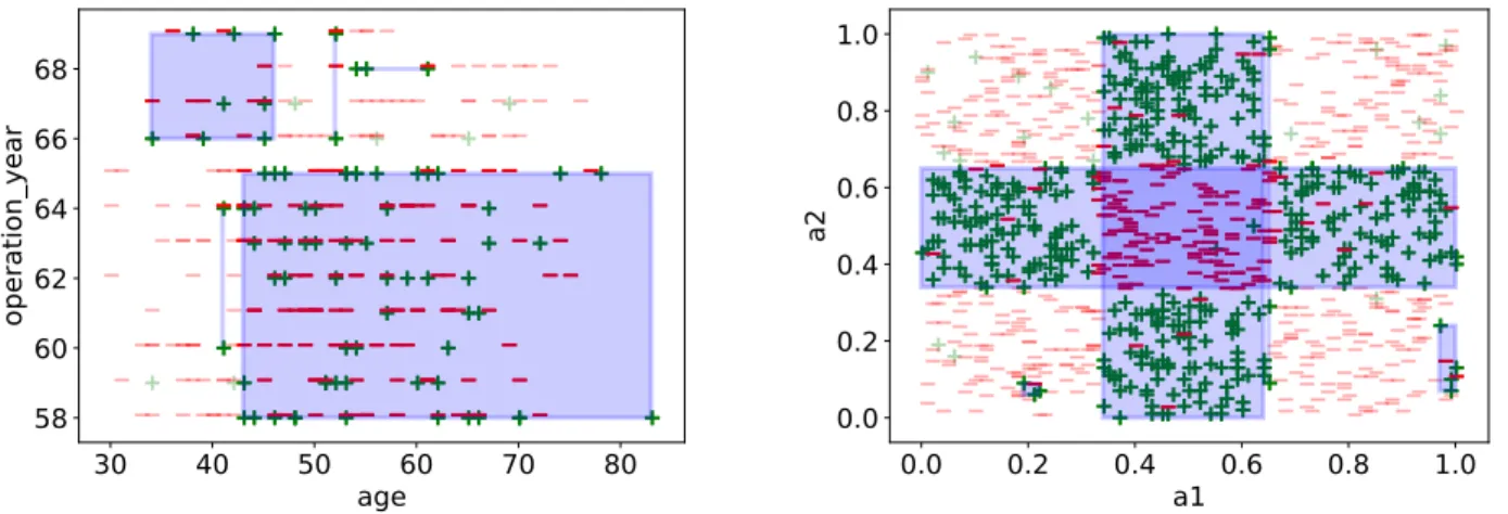
Table III reports a subgroup set of size k= 5 returned by
FSSD when executed on Haberman (D11). This results set covers210/306≈68.6%records of the dataset, with atpr≈ 92.6%and af pr≈0.6. TheWRAccof the set equals0.063. Notice that the identified subgroups are completely disjoint. This example demonstrates the ability of FSSD to uncover a subgroup set that is both discriminant and diversified (see Fig. 2 (left)). It is worth mentioning that FSSD can return overlapping subgroups as depicted in Fig. 2(right).
In order to evaluate the quality of FSSD’ results, we compute the approximation ratioρofFSSDfor the benchmark datasets. This requires to retrieve the ground truth (the optimal solution) for each of the 15 datasets. In order to make the calculation of the ground truth computationally possible, we have reduced the number of attributes. We specify the number of considered attributes for each dataset in its affiliated id. For example, D07-4 refers to the7thdataset and the number of at-tributes is4. Attributes are selected in the following order: first, categorical, and then, numerical. Categorical (resp. numerical) attributes are sorted in an ascending order according to the size of their domain. Table IV reports the results. For most datasets, the approximation ratio is very high.FSSDsucceeds to approximate the ground truth by at least 87% for all the datasets except for D10-3, where the ratio is acceptable (62%). Table V presents the time and memory usage of FSSD
and the BASELINE on all the datasets. The number of attributes is limited so that theBASELINE succeeds to mine the subgroup set in the limit of 30 minutes and without exceeding the machine memory limit. FSSD is faster than the BASELINE in all the configuration. Furthermore, FSSD
consumes significantly less memory than theBASELINE(10 times less in average). The memory usage of theBASELINEis considerably impacted by the number of local subgroups, since it needs to store their complete list in order to process them.
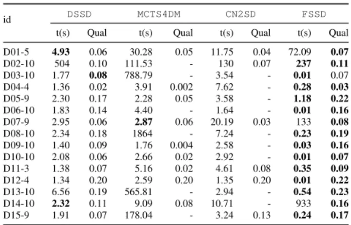
We compareFSSD(Depthmax=8) against the competitive approaches: DSSD (Depthmax=8, BeamWidth=5, j=10000 and coverBeamMultiplier=0.9), MCTS4DM (nbiter=50000
and maxRedundancy=0.25), and CN2-SD (Depthmax=8,
BeamWidth=50 andmin sup pos≥ |G+|/10). We report in
Table VI the runtime and quality of results for each approach on the benchmark datasets. For each dataset, we limit the number of attributes to the maximum number so that the four
Subgroup Intent support WGain
“age∈[43,83]∧operation year∈[58,65]” 179 0.041 “age∈[34,46]∧operation year∈[66,69]” 20 0.009 “age∈[54,61]∧operation year∈[68,68]” 4 0.006 “age∈[41,41]∧operation year∈[60,64]” 3 0.004 “age∈[52,52]∧operation year∈[66,69]” 4 0.003
TABLE III: A subgroup set of size 5, W RAcc ≈ 0.063
and support = 210 identified by FSSD in the dataset D11
projected on two out of three attributes.
id ρ id ρ id ρ id ρ
D01-1 99.7% D05-1 100% D09-5 99.7% D13-7 99.6%
D02-3 100% D06-1 90.54% D10-3 62.2% D14-1 100%
D03-7 87.3% D07-4 99.66% D11-1 100% D15-4 100%
D04-2 100% D08-7 99.62% D12-1 100%
TABLE IV: Approximation ratiosρof the Top3 obtained after running FSSDon each of the15reduced datasets.
id BASELINE FSSD t(s) M(MiB) t(s) Mem.(MiB) D01-5 0.37 22.73 0.21 15.34 D02-10 120.31 426.16 8.70 40.09 D03-10 34.37 37.10 0.09 9.13 D04-4 0.77 25.60 0.29 1.55 D05-9 2.63 103.52 0.06 2.58 D06-10 38.01 23.98 0.04 5.51 D07-9 97.54 2556.15 45.62 7.42 D08-10 3.76 77.22 0.26 3.33 D09-10 34.46 338.61 0.06 2.32 D10-10 11.89 26.11 0.07 9.46 D11-3 33.78 1141.01 7.16 2.58 D12-4 15.78 341.79 0.02 1.29 D13-10 149.25 457.50 3.96 33.52 D14-10 36.97 1533.13 17.77 4.08 D15-9 2.68 20.77 0.27 2.06
TABLE V: Comparison of the runtime -t(s)- and memory consumption -Mem.(MiB)- of FSSD vs. BASELINE for a Top5 subgroup set discovery task on the benchamrk datasets.
id DSSD MCTS4DM CN2SD FSSD t(s) Qual t(s) Qual t(s) Qual t(s) Qual D01-5 4.93 0.06 30.28 0.05 11.75 0.04 72.09 0.07 D02-10 504 0.10 111.53 - 130 0.07 237 0.11 D03-10 1.77 0.08 788.79 - 3.54 - 0.01 0.07 D04-4 1.36 0.02 3.91 0.002 7.62 - 0.28 0.03 D05-9 2.30 0.17 2.28 0.05 3.58 - 1.18 0.22 D06-10 1.83 0.14 4.40 - 1.64 - 0.01 0.16 D07-9 2.95 0.06 2.87 0.06 20.19 0.03 133 0.08 D08-10 2.34 0.18 1864 - 7.24 - 0.23 0.19 D09-10 1.40 0.09 1.76 0.004 2.58 - 0.03 0.16 D10-10 2.08 0.06 2.66 0.02 2.92 - 0.01 0.07 D11-3 1.38 0.07 5.16 0.02 4.61 0.08 0.35 0.09 D12-4 1.34 0.20 2.59 0.20 1.35 0.20 0.01 0.22 D13-10 6.56 0.19 565.81 - 2.94 - 0.54 0.23 D14-10 2.32 0.11 9.09 0.08 10.71 - 933 0.16 D15-9 1.91 0.07 178.04 - 3.24 0.13 0.24 0.17
TABLE VI: Comparison of the runtime and qualities of the Top5 identified subgroups set byFSSD,DSSD,MCTS4DMand
CN2SD. ‘-’ corresponds to the cases when an algorithm fails to find a subgroup set with a strictly positive quality.
algorithms succeed to finish within one hour.FSSDprovides the best qualities for all the datasets except D03, where
DSSD performs better. Particularly, the difference is notable when comparing with CN2-SD and MCTS4DM. Regarding the runtime,FSSDis generally faster thanDSSD,MCTS4DM, andCN2-SDin most configurations except for D01 and D14 whereFSSD managed to find a better subgroup set in terms of the quality.
VII. CONCLUSION
We introduced in this paper a novel problem of diverse subgroup set discovery where both discriminative power and
30
40
50
60
70
80
age
58
60
62
64
66
68
operation_year
0.0
0.2
0.4
0.6
0.8
1.0
a1
0.0
0.2
0.4
0.6
0.8
1.0
a2
Fig. 2: (left)subgroup set found for datasetD11illustrating Table III, (right)subgroup set found for a synthetic dataset with two numerical attributes. One can see that almost all positive instances are covered by the subgroup set.
diversity of the subgroup set are incorporated into the same measure (i.e. quality of subgroups union). We proposed then
FSSD , a parameter-free and memory efficient greedy algo-rithm approximating the solution of the proposed problem.
FSSDexploits closure operators and tight optimistic estimates on the marginal contributions of SD-compatible measures to efficiently explore and prune unpromising areas of the search space. We shown that unfortunately, for many SD-compatible measures like WRAcc, greedy algorithms cannot provide guarantees (lower bound) on the approximation ratio to the best possible solution. Nonetheless, empirical study gave evidence that FSSD (1) is a time and memory efficient algorithm, (2) is able to provide a diverse and high quality subgroup set and (3) provides a judicious trade-off between the runtime and the quality compared to the state-of-the-art approaches. A further improvement of FSSD performance may be achieved if only class-relevant patterns are sought. This requires a polynomial space and output-polynomial time algorithm for enumerating such patterns, which remains an open problem [18]. Other open questions that need to be further investigated are the following: is there an algorithm that ensure approximation guarantees for Problem III-C in a tractable way, i.e. is Problem III-C hard to approximate?
Aknowledgement. This work has been partially supported by the projectContentCheck ANR-15-CE23-0025funded by the French National Research Agency, the Association Nationale Recherche Technologie (ANRt) French program. The authors would like to thank the reviewers for their valuable remarks.
REFERENCES
[1] Rakesh Agrawal, Tomasz Imielinski, and Arun N. Swami. Mining association rules between sets of items in large databases. InACM SIGMOD, pages 207–216. ACM Press, 1993.
[2] Martin Atzm¨uller and Frank Puppe. Sd-map - A fast algorithm for exhaustive subgroup discovery. InPKDD 2006, pages 6–17, 2006. [3] Adnene Belfodil, Sylvie Cazalens, Philippe Lamarre, and Marc Plantevit.
Flash points: Discovering exceptional pairwise behaviors in vote or rating data. InECML/PKDD, 2017.
[4] Aimene Belfodil, Adnene Belfodil, and Mehdi Kaytoue. Anytime sub-group discovery in numerical domains with guarantees. InECML/PKDD (2), volume 11052 ofLecture Notes in Computer Science, pages 500– 516. Springer, 2018.
[5] Tijl De Bie, Kleanthis-Nikolaos Kontonasios, and Eirini Spyropoulou. A framework for mining interesting pattern sets.SIGKDD Explorations, 12(2):92–100, 2010.
[6] Mario Boley, Claudio Lucchese, Daniel Paurat, and Thomas G¨artner. Direct local pattern sampling by efficient two-step random procedures. InKDD, pages 582–590. ACM, 2011.
[7] Guillaume Bosc, Jean-Franc¸ois Boulicaut, Chedy Ra¨ıssi, and Mehdi Kaytoue. Anytime discovery of a diverse set of patterns with monte carlo tree search. Data Min. Knowl. Discov., 32(3):604–650, 2018. [8] Bj¨orn Bringmann and Albrecht Zimmermann. The chosen few: On
identifying valuable patterns. InICDM, pages 63–72, 2007.
[9] Peter Clark and Tim Niblett. The CN2 induction algorithm. Machine Learning, 3:261–283, 1989.
[10] Guozhu Dong and Jinyan Li. Efficient mining of emerging patterns: Discovering trends and differences. InKDD, pages 43–52. ACM, 1999. [11] Usama M. Fayyad, Gregory Piatetsky-Shapiro, and Padhraic Smyth. From data mining to knowledge discovery in databases. AI Magazine, 17(3):37–54, 1996.
[12] Johannes F¨urnkranz and Peter A. Flach. ROC ’n’ rule learning - towards a better understanding of covering algorithms. Machine Learning, 58(1):39–77, 2005.
[13] B. Ganter and R. Wille.Formal Concept Analysis. Springer, 1999. [14] Bernhard Ganter and Sergei O. Kuznetsov. Pattern structures and their
projections. InICCS, pages 129–142, 2001.
[15] Gemma C. Garriga, Petra Kralj, and Nada Lavrac. Closed sets for labeled data. InPKDD, pages 163–174, 2006.
[16] Gemma C. Garriga, Petra Kralj, and Nada Lavrac. Closed sets for labeled data. Journal of Machine Learning Research, 9:559–580, 2008. [17] Liqiang Geng and Howard J. Hamilton. Interestingness measures for
data mining: A survey. ACM Comput. Surv., 38(3):9, 2006.
[18] Henrik Grosskreutz. Class relevant pattern mining in output-polynomial time. InSDM, pages 284–294. SIAM / Omnipress, 2012.
[19] Henrik Grosskreutz, Stefan R¨uping, and Stefan Wrobel. Tight optimistic estimates for fast subgroup discovery. In ECML/PKDD 2008, pages 440–456, 2008.
[20] Tias Guns, Siegfried Nijssen, and Luc De Raedt. Evaluating pattern set mining strategies in a constraint programming framework. InPAKDD, pages 382–394, 2011.
[21] Tias Guns, Siegfried Nijssen, and Luc De Raedt. k-pattern set mining under constraints. IEEE TKDE., pages 402–418, 2013.
[22] Jon Hills, Luke M. Davis, and Anthony Bagnall. Interestingness measures for fixed consequent rules. InIDEAL, pages 68–75. Springer, 2012.
[23] Frederik Janssen and Johannes F¨urnkranz. On trading off consistency and coverage in inductive rule learning. In LWA, volume 1/2006
of Hildesheimer Informatik-Berichte, pages 306–313. University of Hildesheim, Institute of Computer Science, 2006.
[24] Roberto J. Bayardo Jr. and Rakesh Agrawal. Mining the most interesting rules. InKDD, pages 145–154. ACM, 1999.
[25] Mehdi Kaytoue, Sergei O. Kuznetsov, and Amedeo Napoli. Revisiting Numerical Pattern Mining with Formal Concept Analysis. InIJCAI, pages 1342–1347, 2011.
[26] Mehdi Khiari, Patrice Boizumault, and Bruno Cr´emilleux. Constraint programming for mining n-ary patterns. InCP 2010, pages 552–567, 2010.
[27] Willi Kl¨osgen. Explora: A multipattern and multistrategy discovery assistant. InAdvances in Knowledge Discovery and Data Mining, pages 249–271. 1996.
[28] Arno J. Knobbe and Eric K. Y. Ho. Pattern teams. InPKDD, pages 577–584, 2006.
[29] Sergei O. Kuznetsov. Learning of simple conceptual graphs from positive and negative examples. InPKDD, pages 384–391, 1999. [30] Nada Lavrac, Peter A. Flach, and Blaz Zupan. Rule evaluation measures:
A unifying view. InILP, volume 1634 ofLecture Notes in Computer Science, pages 174–185. Springer, 1999.
[31] Nada Lavrac, Branko Kavsek, Peter A. Flach, and Ljupco Todorovski. Subgroup discovery with CN2-SD. JMLR, pages 153–188, 2004. [32] Florian Lemmerich, Mathias Rohlfs, and Martin Atzm¨uller. Fast
dis-covery of relevant subgroup patterns. InFLAIRS, 2010.
[33] Philippe Lenca, Patrick Meyer, Benoˆıt Vaillant, and St´ephane Lallich. On selecting interestingness measures for association rules: User oriented description and multiple criteria decision aid. European Journal of Operational Research, 184(2):610–626, 2008.
[34] Michael Mampaey, Siegfried Nijssen, Ad Feelders, and Arno J. Knobbe. Efficient algorithms for finding richer subgroup descriptions in numeric and nominal data. InICDM, pages 499–508, 2012.
[35] Taneli Mielik¨ainen and Heikki Mannila. The pattern ordering problem. InPKDD 2003, pages 327–338, 2003.
[36] George L. Nemhauser, Laurence A. Wolsey, and Marshall L. Fisher. An analysis of approximations for maximizing submodular set functions -I.Math. Program., 14(1):265–294, 1978.
[37] Miho Ohsaki, Shinya Kitaguchi, Kazuya Okamoto, Hideto Yokoi, and Takahira Yamaguchi. Evaluation of rule interestingness measures with a clinical dataset on hepatitis. InPKDD, volume 3202 ofLecture Notes in Computer Science, pages 362–373. Springer, 2004.
[38] Abdelkader Ouali, Albrecht Zimmermann, Samir Loudni, Yahia Lebbah, Bruno Cr´emilleux, Patrice Boizumault, and Lakhdar Loukil. Integer linear programming for pattern set mining; with an application to tiling. InPAKDD 2017, pages 286–299, 2017.
[39] Gregory Piatetsky-Shapiro. Discovery, analysis, and presentation of strong rules. In Knowledge Discovery in Databases, pages 229–248. AAAI/MIT Press, 1991.
[40] Luc De Raedt and Albrecht Zimmermann. Constraint-based pattern set mining. InSDM, pages 237–248. SIAM, 2007.
[41] Matteo Riondato and Fabio Vandin. Misosoup: Mining interesting subgroups with sampling and pseudodimension. InKDD, pages 2130– 2139, 2018.
[42] S. Roman. Lattices and Ordered Sets. Springer New York, 2008. [43] Arno Siebes. Data science as a language: challenges for computer
science - a position paper. I. J. Data Science and Analytics, 6(3):177– 187, 2018.
[44] Arno Siebes, Jilles Vreeken, and Matthijs van Leeuwen. Item sets that compress. InSDM, pages 395–406. SIAM, 2006.
[45] Pang-Ning Tan, Vipin Kumar, and Jaideep Srivastava. Selecting the right interestingness measure for association patterns. InSIGKDD 2002, pages 32–41. ACM, 2002.
[46] Ljupˇco Todorovski, Peter Flach, and Nada Lavraˇc. Predictive perfor-mance of weighted relative accuracy. InPKDD, pages 255–264, 2000. [47] John W. Tukey. Exploratory data analysis. Addison-Wesley series in
behavioral science : quantitative methods. Addison-Wesley, 1977. [48] Matthijs van Leeuwen and Arno J. Knobbe. Diverse subgroup set
discovery. Data Min. Knowl. Discov., 25(2):208–242, 2012.
[49] Geoffrey I. Webb. OPUS: an efficient admissible algorithm for unordered search.J. Artif. Intell. Res., 3:431–465, 1995.
[50] Stefan Wrobel. An algorithm for multi-relational discovery of sub-groups. InPKDD, pages 78–87, 1997.
[51] Tao Zhang. Association rules. In PAKDD, volume 1805 of Lecture Notes in Computer Science, pages 245–256. Springer, 2000.
APPENDIX
A. Problem III-C is NP-Hard.
Before giving the demonstration, let us consider a reformu-lation of Problem III-C presented below in Problem A.
Problem Statement(Problem A). Let be some set of objects
G partitioned intoG+ andG−. Let
S ⊆℘(G)be all possible
subgroups derived w.r.t. some pattern language and letk∈N∗.
Output one subgroup set fromargmaxS⊆S,|S|≤kWRAcc(S)
Problem A can be seen as a simplification of Problem III-C in the sense that (1) it does consider only the special problem of optimizing the WRAcc measure and (2) consider the set of all possible subgroups S as an input rather than as an
intermediary output. Showing that Problem A is NP-hard allows us hence to show that Problem III-C is also NP-hard. Before showing the NP-hardness of Problem A, we recall below the Maximum Cover Problem (MCP) which is an NP-complete problem. The NP-hardness of MCP is a consequence of the NP-hardness of optimizing a submodular set function subject to a cardinality constraint [36].
Problem Statement (MCP). LetG be a finite universe,S⊆
℘(G)andk∈N∗. Finds out a subsetS ⊆Ssuch that|S| ≤k
for which|S
S|is maximized. Formally, output one solution fromargmaxS⊆S,|S|≤k|
S
S|.
Proposition 1. Problem A is NP-hard.
Proof. Consider the following MCP problem with G+ is a
finite set of elements, S+ ⊆℘(G+)and k∈ N∗. We reduce
(in a polynomial-time) this MCP problem to an instance of Problem A as follow: Build a setG s.t. G=G+∪ G−, G+∩
G−=∅ and|G−|=|G+|. Let
S=S+. It is clear that for all
S ⊆S+, we have: WRAcc(S) = 1 2· |G|· [ S
where 2·|G|1 is a constant. Clearly, any solution of this instance of Problem A is also a solution of the MCP problem instance. Hence, since the MCP Problem is NP-hard then Problem A is NP-hard.
Corollary 1. Problem III-C is NP-hard.
B. Greedy algorithm provides no guarantee.
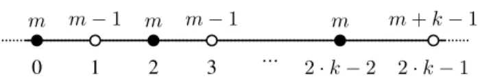
We have investigated in Section IV of the paper that the greedy algorithm provides no guarantee on the approximation ratio. However, in this proof, we considered the language of itemsets. We show here that, still, even for datasets with ex-clusively categorical attributes (or numerical ones), there is no provided guarantee on the approximation ratio. Proposition 2 formalizes this observation.
Proposition 2. ∀ > 0, one can build an instance of Prob-lem III-C such that all the attributes are categorical and solution Sgreedy outputted from Algorithm 1 (i.e. greedy
m−1 m−1
m m m m+k−1
0 1 2 3 ... 2·k−2 2·k−1
Fig. 3: Inexistence of approximation guarantee by the greedy algorithm for numerical datasets (Proposition 2 proof)
Proof. Let us build a parametric instance of Problem III-C wherekis the cardinality constraint and the optimized measure is the WRAccmeasure. Let be m∈N∗, we build the dataset
(G,A)as depicted in Fig. 3. That is:G={gi}0≤i<2·k·mand
A = {a} with a is numerical. The black (resp. white) dots refer to elements in G+ (resp. in G−). We write below each
dot the value of the attributeaand above the dot the number of elements having the same value. For instance, in this dataset, there ismpositive instances having for value0on attributea
followed by m−1 negative instances having for value 1, ... followed by m positive instances having for value 2·k−2
followed by m+k−1 negative instances having for value
2·k−1. It is clear that there isk·mpositive instances andk·m
negative instances. Since the used patterns are interval patterns, withkis the cardinality constraints one can build thek-sized optimal subgroup set S∗ for which WRAcc(S∗) = 0.25 is
optimal (i.e. regroups subgroups associated to constraints0≤ a≤0,2≤a≤2, ... ,2·k−2≤a≤2·k−2). Subgroup setS∗
is optimal since its true positive rate is1and false positive rate is0. That is: it takes all positive instances without covering any negative one. However, one can easily show that the greedy algorithm will output 1-sized subgroup setSgreedy containing
the extent of pattern0≤a≤2·k−2since that this subgroup is the optimal one w.r.t.WRAcc. Hence:WRAcc(Sgreedy) =
0.25·1−(k−1)k··(mm−1). Thus, ρ(Sgreedy) = k+mk·m−1. It is
easy to see now that for all >0 one can always computek
andm such thatρ(Sgreedy)< .
Please note that this proof consider also categorical at-tributes. Indeed, one can transform the numerical dataset
(G,{a})used here to the categorical dataset (G,AC) where
AC ={ai|i∈0..2·k−1} s.t. the range of eachai is given
by Rai ={“≤i”,“ > i”}. If an objectg ∈ G has a(g) =i
in the first dataset then it has aj(g) = “≤j” for all j ≥i
and aj(g) = “> j” for j < i. It is clear that the subgroups
induced by(G,AC)are exactly the same as those induced the
numerical dataset (G,{a}).
One can follow an equivalent reasoning for other SD-compatible measures such as the measures highlighted inbold
in Table VII.
C. Quality measures in SD
Following the notations presented in Sec. II, Table VII presents different quality measures that are used in subgroup discovery. Except the support and the false positive rate, all these quality measures are SD-Compatible following Defi-nition 1. Please note that measures are regrouped in blocs. Each bloc refer tocompatible measures, i.e. measures ordering subgroups in the same way (see Definition 2.2 in [12]).
In order to compute an optimistic estimate (see Definition 4) for these measures, one can follow Theorem 1 where the false positive rate of the subgroup (x) is replaced by 0. The measures highlighted in bold refer to the measure having a non constant optimistic estimate.
Measure Definition
False Positive Rate x:=f pr(t) =|t∩ G−|/|G−| True Positive Rate y:=tpr(t) =|t∩ G+|/|G+|
Positive Prevalence α:=|G+|/|G|
Dataset size n:=|G|
Relative Support [1] s:=α·y+ (1−α)·x
Precision/Confidence [1] p:=α·y/s
Growth Rate [10] [(1−α)/α]·[p/(1−p)] =y/x
Ganascia index [22] 2p−1
Sebag-Schoenaur [22] p/(1−p)
ECE rate [22] 2−1/p
Ohsakis Conviction [37] (1−α)2/(1−p)
Lift [22] p/α
Mutual information [22] log(p/α)
One way support [17] p·log(p/α)
Added Value [30] p−α Certainty Factor [22] (p−α)/(1−α) Brin’s Conviction [22] (1−α)/(1−p) Zhang [51] (y−x)/sup{y, x} Odds Ratio [45] Ω := [y·(1−x)]/[x(1−y)] Yule’s Q [45] (Ω−1)/(Ω + 1) Yule’s x [45] √Ω−1/√Ω + 1 Least contradiction[17] [α·y−(1−α)·x]/α Accuracy[17] α·y−(1−α)·x+ (1−α) WRAcc[30] α·(1−α)·(y−x) Informedness[4] y−x Binomial Test[34] α·(1−α)·(y−x)/√s Kl¨osgenω(ω∈[0,1]) [23] α·(1−α)·sω−1·(y−x) Linear correlation[45] p [(α·(1−α))/(s·(1−s))]·(y−x) Cohen’s kappa(κ)[45] κ:= 2α·(1−α)(y−x)/[α+(1−2α)·s] Cosine/G-Measure[17] y/p [y+ ({1/α} −1)·x] m-estimate(m >0) [12] α·[y+m/n]/[α·y+ (1−α)·x+m/n] Discriminativity[6] n2·α·(1−α)·y·(1−x) Fβ(β∈[0,+∞)) [23] [(1 +β2)·y]/[y+ ({1/α} −1)·x+β2]
TABLE VII: Quality of a subgroupt using its false positive ratex, its true positive ratey, positive prevalence αand the dataset sizen.