Zhang, R., Chen, W., Hsu, T., Yang, H. and Chung, Y. (2017)
'ANG - a combination of Apriori and graph computing
techniques for frequent itemsets mining’,
The Journal of
Supercomputing
. doi: 10.1007/s11227-017-2049-z.
The final publication is available at Springer via
http://dx.doi.org/10.1007/s11227-017-2049-z
ResearchSPAce
http://researchspace.bathspa.ac.uk/
This pre-published version is made available in accordance with publisher
policies.
Please cite only the published version using the reference above.
Your access and use of this document is based on your acceptance of the
ResearchSPAce Metadata and Data Policies, as well as applicable
law:-https://researchspace.bathspa.ac.uk/policies.html
Unless you accept the terms of these Policies in full, you do not have
permission to download this document.
This cover sheet may not be removed from the document.
ANG – A Combination of Apriori and Graph Computing Techniques for Frequent
Itemsets Mining
Rui Zhang
1, Wenguang Chen
2, Tse-Chuan Hsu
3, Hongji Yang
3, and Yeh-Ching Chung
41
Graduate School at Shenzhen, Tsinghua University
Shenzhen 518057, China
Email: [email protected]
2
Department of Computer Science and Technology, Tsinghua University
Beijing 100084, China
Email: [email protected]
3
Centre for Creative Computing, BathSpa University, England
Email: [email protected], [email protected]
4
Research Institute of Tsinghua University in Shenzhen
Shenzhen 518057, China
Email: [email protected]
Abstract
-
The Apriori algorithm is one of the most well-known and widely accepted method for the association rule mining. In Apriori, it uses a prefix tree to representk-itemsets, generates k-itemset candidates based on the
frequent (k-1)-itemsets, and determines the frequent
k-itemsets by traversing the prefix tree iteratively based on the transaction records. When k is small, the execution of Apriori is very efficient. However, the execution of Apriori could be very slow when k becomes large because of the deeper recursion depth to determine the frequent k-itemsets. From the perspective of graph computing, the transaction records can be converted to a graph G (V, E), where V is the set of vertices of G that represents the transaction records and E is the set of edges of G that represents the relations among transaction records. Each k-itemset in the transaction records will have a
corresponding connected component in G. The number of
vertices in the corresponding connected component is the support of the k-itemset. Since the time to find the corresponding connected component of a k-itemset in G is
constant for any k, the graph computing method will be very
efficient if the number of k-itemsets is relatively small. Based on Apriori and graph computing techniques, a hybrid method, called ANG (Apriori and Graph Computing), is proposed to compute the frequent itemsets. Initially, ANG uses Apriori to compute the frequent k-itemsets and then switches to the graph computing method when k becomes large (where the number of k-itemset candidates is relatively small). The experimental results show that ANG outperforms both Apriori and the graph computing method for all test cases.
Keywords: Apriori; Graph Computing; Frequent Itemset Mining; Data Mining
1
Introduction
Data mining is to extract the previously unknown and potentially useful information from a large database [15, 17, 21, 22, 24, 32]. It is the core process of the knowledge
discovery of database [24]. The association rule mining is one of the most important techniques in data mining. The association rule was first proposed in supermarket sales [1]. A supermarket collects a lot of transaction records. The owner wants to find useful information from transaction records to help decision makers draw up sale plans. Information such as certain groups of items are consistently purchased together is interesting. The managers could use the information to adjust store layouts, arrange cross selling, and so on.
A transaction record contains a set of items, where an item means a product. Let I be the set of all items. An association rule may like X→Y, where X, Y⊂I and X∩ Y = ∅.
For example, users who buy milk and bread may also buy butter. We say X = {milk, bread} → Y = {butter} is an association rule if the confidence of X and Y, denoted as
confidence(X, Y) = support (X)/support(X∪ Y), (1)
is greater than the minimum confidence, where support(X) is the number of transaction records that contains X and the minimum confidence is a user-defined threshold. Given a set of transaction records, there may exist a large number of useless association rules in which the supports of X and Y are small although their confidences are large. To eliminate those useless association rules, the association rule mining, in general, is divided into 2 steps. The first step is to find all frequent itemsets whose supports are greater than the minimum support. This step is also known as frequent itemset mining (FIM). The second step is to produce all association rules based on Equation (1) for all frequent itemsets found in the first step. The overall performance of association rule mining is mainly depending on the first step since the second step is easy.
The Apriori algorithm is one of the most well-known and widely accepted method to compute FIM [15, 17, 21, 22, 24, 32]. It uses a prefix tree to represent frequent itemsets [3, 4]. In the prefix tree, each node in the kth level represents a set of
k-itemsets. To avoid useless association rules research, Apriori first generates k-itemset candidates based on the frequent
(k-1)-itemsets. Then, it traverses the prefix tree iteratively based on the transaction records to determine whether a
k-itemset candidate is frequent. When k is small, the execution of Apriori is very efficient. However, the execution of
Apriori could be very slow when k becomes large due to the
deeper recursion depth to determine the frequent k-itemsets. The graph computing is a technique to process a set of large-scale data that can be represented as a graph. Many applications, such as breadth-first search, page rank, connected components, shortest paths, etc., can be implemented by using the graph computing method. From the perspective of graph computing, a set of transaction records can be treated as a graph G = (V, E), where V is the set of vertices of G that represents the transaction records and E is the set of edges of G that represents the relations among transaction records. Two vertices have an edge associated with them if the corresponding transaction records satisfied the condition specified by the relation. For the association rule mining, the relation can be specified as two transaction records have the k items in common, where k = 1, …, |I| and I
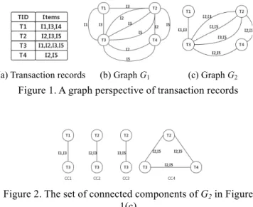
is the set of all items in transaction records. An example of such perspective is shown in Figure 1. In Figure 1(a), a set of transaction records is given. Figure 1(b) shows the corresponding graph G1 in which two transaction records have
1 item in common. Figure 1(c) shows the corresponding graph G2 in which two transaction records have 2 items in
common.
(a) Transaction records (b) Graph G1 (c) Graph G2
Figure 1. A graph perspective of transaction records
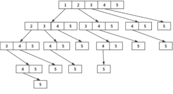
Figure 2. The set of connected components of G2 in Figure 1(c)
Let D be a set of transaction records and Gk be the
corresponding graph of D with value k. From Gk, we can
obtain a set of connected components Ck in which any two
transactions in a connected component have the same k items in common, that is, each k-itemset in D has a corresponding connected component in Ck. The support of a k-itemset
happens to be the number of vertices in the corresponding connected component. Therefore, to use the graph computing method to determine the frequent k-itemsets of D, we only need to compute the number of vertices in each connected components of Ck. If the support is greater than a threshold (minimum support), then this k-itemset is frequent. The performance of using the graph computing method for FIM is determined by the number of connected components in Ck.
Given the graph G2 shown in Figure 1(c), the set of connected
components of G2 is shown in Figure 2.
In Apriori, when k is small, the number of k-itemset candidates could be very huge. If the graph computing method is applied to determine the frequent k-itemsets based on these k-itemset candidates, its execution will be very slow. On the opposite, when k is large, the number of k-itemset candidates will be small. The calculation of frequent
k-itemsets will be very efficient if the graph computing method is applied. Since Apriori is efficient when k is small while the graph computing method is efficient when k is large, in this paper, we propose a hybrid method, called ANG (Apriori and Graph Computing), by combining the advantages of these two methods for FIM. Initially, ANG uses Apriori to perform FIM and then switches to the graph computation
method when k becomes large. We have derived a formula to
determine the switch from Apriori to the graph computing method (this will be described in section 3.3 in detail).
To evaluate ANG, we compared its performance with that of Apriori, DHP (directed hashing and pruning) [23], and the graph computing method. The experimental results show that ANG outperforms Apriori, DHP, and the graph computing method for all test cases. The contributions of this paper are as follows:
1. We have formulated the FIM problem as a graph computing problem.
2. We have proposed a hybrid method, ANG, based on
Apriori and the graph computing method to compute FIM efficiently.
The rest of the paper is organized as follows. Section 2 introduces some graph computing structures and some FIM methods. Section 3 introduces ANG in details. The experimental results are given in section 4.
2
Related Work
Many graph computing techniques have been proposed in the literature [5-10, 14, 16, 18-20, 25-30, 33-35]. They can be divided into two categories, single node graph computing techniques [10, 14, 16, 18, 25-27, 30, 33, 34] and distributed graph computing techniques [5, 7- 9, 19, 20, 31, 35].
In GraphChi [14], the authors proposed a graph computing structure in a single node system. It is a disk-based system to compute graphs with billions of edges from disk by using a novel parallel sliding windows method. GridGraph [34] decomposes graphs into vertex chunks and edge blocks using a 2-level hierarchical partition. It uses a novel dual sliding windows method to process graphs. Ligra [26] is a lightweight in-memory graph computing system. In Ligra, the memory requirement is critical since a graph must be in the memory before processing. Ligra+ [27] is a successor of Ligra by using compression techniques to reduce the size of a graph. GraphBuilder [13] provides a scalable framework for graph loading, extraction, and transformation.
Pregel [20] is a distributed programming framework for graph computing by providing a set of APIs. It uses a synchronous superstep model to synchronize the execution of nodes among a distributed computing environment.
Distributed GraphLab [19] and PowerGraph [8] are graph computing frameworks for data mining and machine learning algorithms with large-scale data.
Apriori was proposed in [1, 2]. It has been widely discussed in [3, 4, 12, 15, 17, 21-24, 32]. In [3, 4], the authors proposed an implementation of Apriori by using the prefix tree. In [15, 17, 21, 22, 24], some parallel and distributed implementations of Apriori with MapReduce [7] were proposed. In [12], the authors implemented Apriori based on Hadoop. In [23], the authors provide a hash-based algorithm, DHP, for mining association rules. The difference between this method and Apriori is the way to generate the frequent itemset candidates. In Apriori, a prefix tree is used to generate the frequent itemset candidates while in DHP, a hash table is used. In [24], the infrequent itemsets mining based on MapReduce was discussed. In [32], the authors proposed a hash-based method to discover the maximal frequent itemsets.
3
The Proposed Method
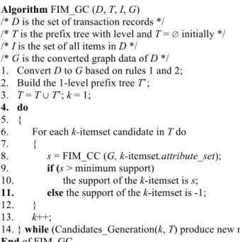
3.1Apriori AlgorithmThe Apriori algorithm used in this paper is based on the work proposed in [4]. In [4], it uses the prefix tree to express all subsets of a set of items. Based on the prefix tree, the frequent k-itemsets can be calculated iteratively. Let I be a set of items, Sk be all subsets of I with k items, and |I| = n. An n level prefix tree T can be used to represent all subsets of
I, where the node in the first level of T contains S1, nodes in
the second level of T contain S2, nodes in the third level of T
contain S3, and so on. An example of using the prefix tree to
represent all subsets of I with n = 5, is shown in Figure 3.
Figure 3. A prefix tree for 5 items
Let D be a set of transaction records and I be a set of items. To calculate all the frequent k-itemsets of D based on the prefix tree, the execution of Apriori is composed of two phases, initial and iterative.
Phase 1. In the initial phase where k = 1, the frequent 1-itemsets are calculated by scanning D once to obtain the support of each 1-itemset. If the support of a 1-itemset is greater than the minimum support, the 1-itemset is a frequent 1-itemset. Otherwise, the support of the 1itemset is set to -1 to indicate that the itemset is not a frequent one.
Phase 2. In the iterative phase where k > 1, Apriori uses the frequent (k-1)-itemsets generated in the (k-1)th level of the prefix tree to generate k-itemset candidates. To determine
whether a k-itemset candidate is frequent, Apriori traverses the prefix tree iteratively based on the transaction records to get the support of each k-itemset candidate. If the support of a
k-itemset candidate is greater than the minimum support, then it is a frequent k-itemset. Otherwise, the support of the
k-itemset is set to -1.
The Apriori algorithm is give as follows:
__________________________________________________
Algorithm Apriori (D, I, T)
/* D is the set of transaction records */ /* I is the set of all items in D */
/* T is the prefix tree with level and T = ∅ initially */
/* Initial phase */
1. Build the 1-level prefix tree T’; 2. T = T ∪T’;
3. Scan D once to obtain the support of each 1-itemset; 4. if (the support of a 1-itemset <= minimum support) the
support of the 1-itemset is set to -1; /* Iterative phase */
5. k=2;
6. Candidates_Generation (k, T);
7. while (Candidates_Generation (k, T) produce new nodes)
8. { 9. T = Apriori_c (k, D, T); 10. k++; 11. Candidates_Generation (k, T); 12.} End of Apriori Algorithm Candidates_Generation (k, T) /* T is the prefix tree */
1. let p and q be 2 frequent (k-1)-itemsets;
2. if (the items of p and q are the same except the last one)
3. {
4. Add a k-itemset candidate exc with the same (k-2) items and different 2 last items to the corresponding position in the kth level of T;
5. if (one of the subset of exc with k-1 items is not a frequent (k-1)-itemset) the support of exc is set to -1;
6. }
End of Candidates_Generation
Function Apriori_c (k, D, T)
/* D is the set of transaction records */ /* T is the prefix tree with level = k-1 */
1. Build the k-level of prefix tree T’ based on T; 2. For each transaction record r in D do
3. {
4. Use r to traverse T’ iteratively;
5. If the traverse reached a leaf node of T’, the support of the corresponding k-itemset is increased by 1;
6. }
7. if (the support of a k-itemset <= minimum support) the support of the k-itemset is set to -1;
8. return T’;
End of Apriori_c
The time complexity of Apriori is O(k2 Í |D| Í
𝐶( 𝐼 , 𝑖))
'()
*+) based on the method proposed in [4]. An
example of using Algorithm Apriori(D, I, T) for FIM is shown in Figure 4. In Figure 4(a), a set of transaction records D = {T1, T2, T3, T4} is given and I = {I1, I2, I3, I4, I5}. In the
initial phase, we can obtain the 1-itemset candidates, the frequent 1-itemsets with support > 1, and the one-level prefix tree as shown in Figures 4(b), 4(c), and 4(d), respectively. In the iterative phase, when k = 2, we can obtain the 2-itemset candidates, the frequent 2-itemsets with support > 1, and the
two-level prefix tree as shown in Figures 4(e), 4(f), and 4(g), respectively. When k = 3, the 3-itemset candidates, the frequent 3-itemsets with support > 1, and the three-level
prefix tree are shown in Figures 4(h), 4(i), and 4(j), respectively.
(a) Transaction records
(b) 1-itemset candidates (c) Frequent 1-itemsets (d)1-level prefix tree
(e) 2-itemset candidates (f) Frequent 2-itemsets (g) 2-level prefix tree
(h) 3-itemset candidates (i) Frequent 3-items (j) 3-level prefix tree Figure 4. An example of using Apriori for FIM
3.2Graph Computing Method
To use the graph computing method to compute FIM, the process can be divided into two phases, converting phase and
computing phase:
Phase 1. In the converting phase, we convert the transaction records to graph data. Given a set of transaction records D and a set of all items of D, denoted as I, we can covert D to a graph data G = (V, E) by using the following rules:
Rule 1. For each transaction record r in D, it denotes as a vertex v in V. The vertex ID of v is the record ID of r.
Rule 2. If two transaction records have k items in common, there will be an edge between two vertices and the attributes associated with the edge is the set of IDs of k items, where k = 1, …, |I|.
Phase 2. In the computing phase, we determine the frequent k-itemsets based on G and the prefix tree T. From
G, we can derive Gk that is the corresponding graph of all k-itemsets in D, where k = 1, …, |I|. Since each k-itemset in
D has a corresponding connected component in Ck. The support of a k-itemset is the number of vertices in the
corresponding connected component. Given the k-itemset
candidates in T, to determine whether a k-itemset candidate is frequent, we only need to find the corresponding connected component of the k-itemset candidate in Ck and compute the number of vertices (counter) in the corresponding connected components. If the counter is greater than a threshold (minimum support), then this k-itemset is frequent.
The algorithm to use the graph computing method to calculate the frequent itemsets is given as follows.
__________________________________________________
Algorithm FIM_GC (D, T, I, G) /* D is the set of transaction records */
/* T is the prefix tree with level and T = ∅ initially */
/* I is the set of all items in D */ /* G is the converted graph data of D */ 1. Convert D to G based on rules 1 and 2; 2. Build the 1-level prefix tree T’; 3. T = T ∪T’; k = 1;
4. do
5. {
6. For eachk-itemset candidate inT do
7. {
8. s = FIM_CC (G, k-itemset.attribute_set);
9. if (s > minimum support)
10. the support of the k-itemset is s;
11. else the support of the k-itemset is -1;
12. }
13. k++;
14.} while (Candidates_Generation(k, T) produce new nodes)
End of FIM_GC
Algorithm FIM_CC (G, attribute_set)
1. labels = {0, …, |V-1|} initialized such that labels[i]=i; 2. for each edge e in G do Fe(e, attribute_set);
3. Return the counter of vertices in the connected component;
End of FIM_CC
Function Fv (vertex, new_label)
1. labels[vertex] = new_label;
End of Fv
Function Fe (edge, attribute_set)
1. if (attribute_set is a subset of attributes of edge)
2. { 3. m = min(labels[edge.source], labels[edge.destination]); 4. Fv (edge.source, m); 5. Fv (edge.destination, m); 6. } End of Fe __________________________________________________
In the graph computing method, the converting phase (Phase 1) will be executed only once. Its time complexity is
O(|D|2). In the computing phase, the maximum number of
frequent itemset candidates processed in the kth iteration is
C(|I|,k). The time complexity of this phase is
O( ' 𝐶 𝐼 , 𝑖
*+) *|E|).
3.3ANG Algorithm
The different between the graph computing method and Apriori is the way to compute the support of k-itemset. Apriori uses the transaction records to traverse the prefix tree iteratively to calculate the supports of k-itemset candidates while the graph computing method uses the connected components algorithm to compute the supports of k-itemsets.
When k is small, Apriori can be very efficient. However, Apriori will be very inefficient when k becomes large because of the deeper recursion depth. It indicates that the execution time of Apriori is mainly depending on the level of prefix tree traversed. For the graph computing method, it computes a support of a k-itemset by executing the connected components algorithm once. The time of executing multi-attributes connected components algorithm for different k-itemsets is almost the same. Therefore, the execution time of the graph computing method is mainly depending on the number of
k-itemsets.
In Apriori algorithm, the number of k-itemset candidates, in general, is much less than the number of k-itemsets in the prefix tree. We observe that the number of k-itemset candidates is large when k is small. While k become large, the number of k-itemset candidates decreases sharply. Table 1 shows the number of k-itemset candidates of a set of transaction records with different minimum supports percentage s. The minimum support is defined as s times the number of transaction records. The 1-itemset candidates are the whole items, and the k-itemsets candidates are depending on frequent (k-1)-itemsets. From Table 1, we can see that the number of k-itemset candidates decrease greatly when k > 2.
Table 1. The number of k-itemset candidates
Apriori is very efficient when k is small while the graph computing method with the prefix tree can accelerate the computation of the support of k-itemset candidates when k is large. By using this feature, we propose the ANG algorithm to perform FIM. In ANG, initially the Apriori method is used when k is small. When k is large, the graph computing method is applied. We need to determine the value of k such that the execution can be switched from the Apriori method to the graph computing method.
Let Ni be the number of items in the ith transaction record, CAk be the number of k-itemset candidates, trk be the time of one transaction record traversing a prefix tree with depth k, tck be the time to execute the connected components
algorithm with k items. The time to compute the support of
k-itemset candidates in Apriori is 𝐶,'-∗ 𝑡0'. The time to
compute the support of k-itemset candidates in the graph computation method is 𝐶𝐴'∗ 𝑡2'. When the time of Apriori
is greater than the time of the graph computation method, we switch to the graph computing method i.e. when the Equation (2) is satisfied.
𝐶(𝑁*, 𝑘) ∗ 𝑡0'> 𝐶𝐴'∗ 𝑡2' (2)
The algorithm of ANG is given as follows.
__________________________________________________
Algorithm ANG (D, T, G)
/* D is the set of transaction records */
/* T is the prefix tree with level and T = ∅ initially */
/* G is the converted graph data of D */ 1. Build the 1-level prefix tree T’; 2. T = T ∪T’;
3. Scan D once to obtain the support of each 1-itemset; 4. if (the support of a 1-itemset <= minimum support) the
support of the 1-itemset is set to -1; 5. k=2;
6. Candidates_Generation (k, T); 7. while (Equation (2) is not satisfied)
8. {
9. Apriori_c (k, D, T);
10. k++;
11. Candidates_Generation (k, T); 12.}
13.while (k-itemset candidates are not empty) 14.{
15. Build k-level prefix tree T’ based on T; 16. for each k-itemset candidate do
17. {
18. s = FIM_CC (G, candidate.attribute_set);
19. if (s < minimum support) support of the k-itemset is set to -1; set corresponding support of k-itemset = s; 20. k++; 21. Candidates_Generation (k, T’); 22. } 23.} End function __________________________________________________ The time complexity of ANG is O(j2 Í |D| Í
𝐶( 𝐼 , 𝑖))
7()
*+) + O( '*+7𝐶 𝐼 , 𝑖 *|E|), where j and k are the
first and the last iterations performed by Algorithm FIM_CC(G, candidate.attribute_set) in Algorithm ANG(D, T,
G), respectively. The execution flow of the ANG algorithm is shown in Figure 5. s = 0.1% s = 0.2% s = 0.3% s = 0.4% 1-itemsets 1000 1000 1000 1000 2-itemsets 318003 274911 242556 200028 3-itemsets 158413 30110 7881 1788 4-itemsets 5493 2719 737 200 5-itemsets 3140 1631 266 53 6-itemsets 1427 826 61 11 7-itemsets 494 303 11 1
Figure 5.The execution flow of the ANG algorithm
4
Experimental Results
To evaluate the performance of ANG, we have implemented ANG algorithm along with Apriori, DHP, and the graph computing method. We use the set of transaction records in [11] as the test sample. The set contains 61100 transaction records and 1000 items. Items in transaction records are uniform distributed, that is, each item has the same influence to the experiment conducted.
Table 1 shows the number of k-itemset candidates in the prefix tree with different minimum support percentages s for the test sample. Tables 2-5 show the execution time (in seconds) of Apriori and the graph computing method for the
k-itemset candidates shown in Table 1. From Tables 2-5, we have the following observation:
Observation 1: If the value of minimum support percentage increases, the time for the graph computing method to determine the frequent itemsets from the k-itemset candidates will be less than that of the Apriori method with smaller k.
For example, if s is 0.1%, the time for the graph computing method to determine the frequent itemsets from the 7-itemset candidates is 247 seconds while that of the Apriori method is 711.11 second. When s is increased to 0.3%, the time for the graph computing method to determine the frequent itemsets from the 5-itemset candidates is 106.4 seconds while that of the Apriori method is 176.29 second.
In ANG, Equation (2) is used to determine when to switch from Apriori to the graph computing method. Given the test sample, in Equation (2), 𝐶(𝑁*, 𝑘) can be computed for a given Niand k. The value of trk is the time for each transaction record to traverse a prefix tree with depth k. The levels traversed for trk and tr(k-1) are k and k-1, respectively. trk can be approximated as trk = tr(k-1) + (tr(k-1)−tr(k−2)) = 2tr(k-1) - tr(k-2). Values of CAkare shown in Table 1, where k= 1, …, 7.
The value of tck can be obtained by executing the connected
component algorithm with k items once.
For the case where s = 0.3% and k = 5, we have
𝐶(𝑁*, 5) = 689419357, tr5 = 2.56μs since tr4 = 2.52μs and tr3 =2.48μs, CA5 is 266, and tc5 = 0.37s. Based on the values
of 𝐶(𝑁*, 5), tr5, CA5, and tc5, the estimated time for the Apriori method and the graph computing method are 176.49 and 98.42 seconds, respectively. Given the test sample and s
= 0.3%, ANG will use the Apriori method to calculate the frequent itemsets when k < 5 and switches to the graph computing method after k ≥ 5 since the condition given in Equation (2) is satisfied.
Tables 6-9 show the estimated execution of Apriori and the graph computing method based on the values of
𝐶(𝑁*, 𝑘), trk, CAk, and tckfor the test sample with s = 0.1%,
0.2%, 0.3%, and 0.4%, respectively. Compare Tables 2-5 and Tables 6-9, we can see that Equation (2) can predict the switching points for ANG accurately for all test cases. Table 10 shows the execution time of Apriori, ANG, and the graph computing method for the test sample. From Table 10, we can see that ANG has the best performance among the three methods compared for all test cases.
Table 2. The execution time (s) of Apriori and the graph computing method for k-itemset candidates with s = 0.1%
Apriori Graph Computing 2-itemsets 8.54 130381.24 3-itemsets 37.16 64949.35 4-itemsets 102.12 2252.12 5-itemsets 232.54 1287.43 6-itemsets 438.68 713.6 7-itemsets 711.11 247
Table 3. The execution time (s) of Apriori and the graph computing method for k-itemset candidates with s = 0.2%
Apriori Graph Computing 2-itemsets 7.58 112713.51 3-itemsets 31.59 12345.15 4-itemsets 88.04 1114.79 5-itemsets 198.78 668.71 6-itemsets 374.29 330.4 7-itemsets 608.63 151.5
Table 4. The execution time (s) of Apriori and the graph computing method for k-itemset candidates with s = 0.3%
Apriori Graph Computing 2-itemsets 7.37 99447.96 3-itemsets 28.65 3231.21 4-itemsets 78.71 302.17 5-itemsets 176.29 106.4 6-itemsets 333.26 30.5 7-itemsets 541.42 7.7
Table 5. The execution time (s) of Apriori and the graph computing method for k-itemset candidates with s = 0.4%
Apriori Graph Computing 2-itemsets 6.41 82011.49 3-itemsets 24.91 733.07 4-itemsets 68.76 82.71 5-itemsets 155.02 21.74 6-itemsets 291.69 6.6 7-itemsets 474.55 1.2
Table 6. The estimated time (s) of Apriori and the graph computing method for k-itemset candidates with s = 0.1%
Apriori Graph Computing 2-itemsets 8.66 108121.02 3-itemsets 37.13 53860.42 4-itemsets 119.11 1977.48 5-itemsets 233.02 1161.8 6-itemsets 439.58 585.07 7-itemsets 691.27 207.48
Table 7. The estimated time (s) of Apriori and the graph computing method for k-itemset candidates with s = 0.2%
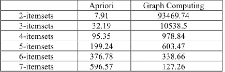
Apriori Graph Computing 2-itemsets 7.91 93469.74 3-itemsets 32.19 10538.5 4-itemsets 95.35 978.84 5-itemsets 199.24 603.47 6-itemsets 376.78 338.66 7-itemsets 596.57 127.26
Table 8. The estimated time (s) of Apriori and the graph computing method for k-itemset candidates with s = 0.3%
Apriori Graph Computing 2-itemsets 7.42 82469.04 3-itemsets 28.62 2758.35 4-itemsets 84.09 265.32 5-itemsets 176.49 98.42 6-itemsets 330.64 25.01 7-itemsets 520.82 4.62
Table 9. The estimated time (s) of Apriori and the graph computing method for k-itemset candidates with s = 0.4%
Apriori Graph Computing 2-itemsets 6.29 68009.52 3-itemsets 24.83 625.8 4-itemsets 74.09 73.44 5-itemsets 154.43 19.61 6-itemsets 294.76 4.51 7-itemsets 464.01 0.42
Table 10. The execution time (s) of Apriori, ANG and the graph computing method
s Apriori ANG Graph Computing 0.1% 1546.15 1032.64 200067.72 0.2% 1324.12 905.69 127710.91 0.3% 1179.69 297.72 103529.93 0.4% 1036.31 145.55 83258.75
In addition to the performance comparison of Apriori, ANG, and the graph computing method, we also compare the performance of ANG with DHP, another method for FIM. Figure 6 shows the execution time of ANG and DHP for the test cases with minimum support from 0.1 to 0.4. From Figure 6, we can see that ANG outperforms DHP for all test cases.
Figure 6.The execution time (s) of ANG and DHP for test cases with different minimum support
5
Conclusions
In this paper, we have shown that how to use the graph computing method to perform frequent itemset mining. We also discussed the advantages and disadvantages of Apriori and the graph computing method when applied them to frequent itemset mining. Based on the discussions, we have proposed a hybrid method, ANG, by taking the advantages of Apriori and the graph computing method for frequent itemset mining. In ANG, initially, Apriori is used to compute the support of k-itemset candidates when k is small. When k
becomes large, the graph computation method is used to compute the support of k-itemset candidates. We have derived a formula to determine when to switch from the Apriori method to the graph computing method. The experimental results show that the formula can predict the switching point accurately and ANG outperforms Apriori, DHP, and the graph computing method for all test cases.
ACKNOWLEDGMENT
The work of this paper is partially supported by Shenzhen City Brach Committee under contract 2016-09.01
References
[1]. Agrawal R, Imielinski T, Swami AN (1993) Mining association rules between sets of items in large databases. In: Proceeding of the SIGMOD’93, pp. 207– 216.
[2]. Agrawal R, Srikant R (1994) Fast algorithms for mining association rules. In: Proceeding of the VLDB’94, pp. 487–499.
[3]. Borgelt, C, Kruse, R (2002) Induction of Association
Rules: Apriori Implementation. In: Compstat.
Physica-Verlag HD, pp. 937-944.
[4]. Borgelt, C (2003). Efficient implementations of apriori and eclat. In: Proc.ieee Icdm Workshop on Frequent Item Set Mining Implementations. ceur Workshop
Proceedings, 90.
[5]. Chen R, Shi JX, Chen YZ, Chen HB (2015) Powerlyra:
Differentiated graph computation and partitioning on skewed graphs. In: Proceedings of the Tenth European Conference on Computer Systems. ACM, pp. 1-15.
[6]. Chen Z, Yang S, Shang Y, Liu Y, Wang F, Wang L, Fu J
(2016) Fragment Re-Allocation Strategy Based on Hypergraph for NoSQL Database Systems. In: International Journal of Grid and High Performance Computing, vol. 8(3), pp. 1-24.
[7]. Dean J, Ghemawat S (2004) MapReduce: Simplified
Data Processing on Large Clusters. In Proc. of the 17th ACM SIGKDD international conference on Knowledge discovery and data mining, pp. 219-228.
[8]. Gonzalez JE, Low YC, Gu HJ, Bickson D, Guestrin C
(2012) PowerGraph: Distributed graph-parallel
computation on natural graphs. In: OSDI, pp. 17-30.
[9]. Gonzalez JE, Xin RS, Dave A, Crankshaw D, Franklin
MJ, Stoica I (2014) GraphX: Graph Processing in a Distributed Dataflow Framework. In: 11th USENIX Symposium on Operating Systems Design and Implementation, pp. 599-613.
[10]. Han WS, Lee S, Park K, Lee JH, Kim MS, Kim J, Yu H
(2013) Turbograph: a fast parallel graph engine handling billion-scale graphs in a single pc. In:
Proceedings of the 19th ACM SIGKDD international conference on Knowledge discover and data mining, ACM, pp. 77-85.
[11]. http://fimi.ua.ac.be/
[12]. https://github.com/solitaryreaper/HadoopApriori
[13]. Jain N, Liao G, Willke TL (2013) GraphBuilder:
scalable graph etl framework. In: First International Workshop on Graph Data Management Experiences and Systems, ACM, pp. 1-6.
[14]. Kyrola A, Blelloch G, Guestrin C (2012) GraphChi: Large-Scale Graph Computation on Just a PC. In: OSDI, vol. 12, pp. 31-46.
[15]. Lin M, Lee P, Hsueh S (2012) Apriori-based frequent itemset mining algorithms on MapReduce. In Proc. ICUIMC, ACM, pp. 26–30.
[16]. Lin Z, Kahng M, Sabrin KM, Chau DHP, Lee H, Kang
U (2014) Mmap: Fast billion-scale graph computation on a pc via memory mapping. In: IEEE International Conference on Big Data, IEEE, pp. 159-164.
[17]. Li N, Zeng L, He Q, Shi Z (2012) Parallel implementation of apriori algorithm based on MapReduce. In: Proc. SNPD, pp. 236–241.
[18]. Low Y, Gonzalez J, Kyrola A, Bickson D, Guestrin C,
Hellerstein JM (2010) GraphLab: A new parallel framework for machine learning. In: Conference on Uncertainty in Artificial Intelligence, pp. 340-349.
[19]. Low Y, Gonzalez J, Kyrola A, Bickson D, Guestrin C,
Hellerstein JM (2012) Distributed GraphLab: A Framework for Machine Learning and Data Mining in the Cloud. In: Proceedings of the VLDB Endowment. pp. 716-727.
[20]. Malewicz G, Austern MH, Bik AJ, Dehnert JC, Horn I,
Leiser N, Czajkowski G (2010) Pregel: a system for large-scale graph processing. In: Proceedings of the
ACM SIGMOD International Conference on
Management of data, ACM, pp. 135-146.
[21]. Moens S, Aksehirli E, Goethals B (2012) Frequent Itemset Mining for Big Data. In: IEEE International Conference on Big Data, IEEE, pp. 111-118.
[22]. Othman Y, Osman H, Ehab E (2012) An efficient implementation of apriori algorithm based on hadoop- MapReduce model. In: International Journal of Reviews in Computing, Vol. 12, pp.57-67.
[23]. Park JS, Chen MS, Yu PS (1995) An Effective
Hash-Based Algorithm for Mining Association Rules. In: Proceedings of the ACM SIGMOD, pp. 175-186.
[24]. Ramakrishnudu T, Subramanyam RBV (2015) Mining Interesting Infrequent Itemsets from Very Large Data based on MapReduce framework. In: International Journal of Intelligent Systems Technologies &
Applications,7(7), 44-49.
[25]. Roy A, Mihailovic I, Zwaenepoel W (2013) X-Stream:
Edge-centric Graph Processing using Streaming Partitions. In: Proceedings of the Twenty-Fourth ACM Symposium on Operating Systems Principles, ACM, pp. 472-488.
[26]. Shun J, Blelloch GE (2013) Ligra: A Lightweight Graph
Processing Framework for Shared Memory. In: ACM SIGPLAN Notices, vol. 48, ACM, pp. 135-146.
[27]. Shun J, Dhulipala L, Blelloch GE (2015) Smaller and Faster: Parallel Processing of Compressed Graphs with Ligra+. In: Proceedings of the IEEE Data Compression Conference (DCC), pp. 403-412.
[28]. Tian J, Zhang H (2016) A Credible Cloud Service Model based on Behavior Graphs and Tripartite Decision-Making Mechanism. In: International Journal of Grid and High Performance Computing, vol. 8(3), pp. 39-57.
[29]. Viswanathan V (2016) Discovery of semantic
associations in an RDF graph using bi-directional BFS on massively parallel hardware. In: International Journal of Big Data Intelligence, vol.3, No.3, pp. 176-181.
[30]. Wang K, Xu G, Su Z, Liu YD (2015) Graphq: Graph query processing with abstraction refinement: scalable and programmable analytics over very large graphs on a single PC. In: USENIX ATC, pp. 387-401.
[31]. Xin RS, Gonzalez JE, Franklin MJ, Stoica I (2013) GraphX: A Resilient Distributed Graph System on Spark. In: First International Workshop on Graph Data Management Experiences and Systems, ACM, p. 2.
[32]. Yong DL, Pan CT, Chung YC (2001) An Efficient
Hash-Based Method for Discovering the Maximal Frequent Set. In: Proceedings of IEEE International
Computer Software and Applications Conference
(COMPSAC), IEEE, pp. 511-516.
[33]. Yuan P, Zhang W, Xie C, Jin H, Liu L, Lee K (2014) Fast Iterative Graph Computation: A Path Centric
Approach. In: High Performance Computing,
Networking, Storage and Analysis, IEEE, pp. 401-412.
[34]. Zhu X, Han W, Chen W (2015) GridGraph: Large-Scale
Graph Processing on a Single Machine Using 2-Level Hierarchical Partitioning. In: USENIX ATC, pp. 375-386.
[35]. Zhu X, Chen W, Zheng W, Ma X (2016) Gemini: A Computation-Centric Distributed Graph Processing System. In: OSDI, pp. 301-316.