Machine learning hyperparameter selection for Contrast Limited Adaptive Histogram Equalization

R E S E A R C H

Open Access

Machine learning hyperparameter

selection for Contrast Limited Adaptive

Histogram Equalization

Gabriel Fillipe Centini Campos

, Saulo Martiello Mastelini

, Gabriel Jonas Aguiar

,

Rafael Gomes Mantovani

, Leonimer Flávio de Melo

and Sylvio Barbon Jr

Abstract

Contrast enhancement algorithms have been evolved through last decades to meet the requirement of its objectives. Actually, there are two main objectives while enhancing the contrast of an image: (i) improve its appearance for visual interpretation and (ii) facilitate/increase the performance of subsequent tasks (e.g., image analysis, object detection, and image segmentation). Most of the contrast enhancement techniques are based on histogram modifications, which can be performed globally or locally. The Contrast Limited Adaptive Histogram Equalization (CLAHE) is a method which can overcome the limitations of global approaches by performing local contrast enhancement. However, this method relies on two essential hyperparameters: thenumber of tilesand theclip limit. An improper hyperparameter selection may heavily decrease the image quality toward its degradation. Considering the lack of methods to efficiently determine these hyperparameters, this article presents a learning-based hyperparameter selection method for the CLAHE technique. The proposed supervised method was built and evaluated using contrast distortions from well-known image quality assessment datasets. Also, we introduce a more challenging dataset containing over 6200 images with a large range of contrast and intensity variations. The results show the efficiency of the proposed approach in predicting CLAHE hyperparameters with up to 0.014 RMSE and 0.935R2values. Also, our method overcomes both experimented baselines by enhancing image contrast while keeping its natural aspect.

Keywords: Local contrast enhancement, Contrast Limited Adaptive Histogram Equalization, CLAHE parameter determination, Hyperparameter selection

1 Introduction

Image enhancement consists of image quality improve-ment processes, allowing a better visual and computa-tional analysis [1]. It is widely used in several applications due to its capability to overcome some of the limitations presented by image acquisition systems [2]. Deblurring, noise removal, and contrast enhancement are some exam-ples of image enhancement operations. The idea behind contrast enhancement is to increase the dynamic range of the gray levels in the image being processed [3]. It plays a major role in digital image processing, computer vision, and pattern recognition [4].

*Correspondence:[email protected]

1_{Electrical Engineering Department, Londrina State University, Rodovia Celso}

Garcia Cid, Londrina 86057-970, Brazil

Full list of author information is available at the end of the article

Besides providing a better visual interpretation by improving the image appearance, the contrast enhance-ment may also be used to improve the performance of succeeding tasks, such as image analysis, object detection, and image segmentation [2,4,5]. In fact, it has contributed in a variety of fields like medical image analysis, high-definition television (HDTV), industrial X-ray imaging, microscopic imaging, and remote sensing [6].

Most of the contrast enhancement techniques are based on histogram adjusts, due to their straight forward and intuitive implementation qualities [5]. A comprehensive review of histogram-based techniques may be found in [6]. These techniques are often categorized in global or local techniques. The use of global contrast enhance-ment may be not suitable for images whose local details are necessary or for images containing varying lighting

conditions. On the other hand, if the process is applied locally, it is possible to overcome those limitations [4,7].

The Contrast Limited Adaptive Histogram Equaliza-tion (CLAHE) [8] is a popular method for local contrast enhancement that has been showing powerful and useful for several applications [4,9,10]. CLAHE has been exten-sively used to enhance image contrast in several computer vision and pattern recognition applications. In the medi-cal field, it was successfully applied in breast ultrasound and mammography image enhancement [11, 12], in cell image segmentation [13,14], in retinal vessel image pro-cessing [15, 16], and in enhancement of bone fracture images [17]. Beyond medical field, CLAHE was applied to enhance underwater images [18,19], to perform fruit seg-mentation in agricultural systems [20, 21], and to assist driving systems to improve vehicle detection [22], traffic sign detection [23], and pedestrian detection [24].

The basic idea of CLAHE consists in performing the histogram equalization of non-overlapping sub-areas of the image, using interpolation to correct inconsistencies between borders [8,25]. CLAHE has also two important hyperparameters: the clip limit (CL) and the number of tiles (NT). The first one (CL) is a numeric value that controls the noise amplification. Once the histogram of each sub-area is calculated, they are redistributed in such a way that its height does not exceed a desired “clip limit.” Then, the cumulative histogram is calculated to perform the equalization [7]. The second (NT) is an inte-ger value which controls the amount of non-overlapping sub-areas: based on its value, the image is divided into several (usually squared) non-overlapping regions of equal sizes. According to [7], for 512×512 images, the number of regions is generally selected to be equal to 64 (NT = [ 8, 8]). Both parameters (CL and NT) are exemplified in Fig.1.

Thus, the main drawback in CLAHE, as reported in [26,27], is an improper hyperparameter selection that leads to decrease in image quality. The authors also state that the quality of the enhanced image depends most on the CL hyperparameter.

Most work relies on fixed hyperparameter values empir-ically chosen to solve a specific problem [20, 28–30]. Nonetheless, an entropy-based method to automatically determine CLAHE’s hyperparameters was proposed in [26]. It takes advantage of the characteristics of two entropy curves (CL per entropy and NT per entropy). The method proposed by the authors determines the CL and NT values as the points with the maximum curvature in each entropy function curve. Obtaining these func-tions requires to calculate the entropy for every CLAHE’s output considering all possible combinations of CL and NT. Although experimental results showed the proposed approach is capable of enhancing the image contrast with low deterioration, the process is computationally

impractical. Calculating the entropy values of all the pos-sible combinations between these hyperparameters is an unfeasible task. Also, the proposed hyperparameter sug-gestion was poorly tested and validated, once only three images were used in their experiments.

A hyperparameter tuning for CLAHE based on multi-objective meta-heuristic was proposed by [25]. In addition to entropy, as proposed in [26], the authors used the Structural Similarity Index (SSIM) to find most promis-ing CLAHE’s hyperparameters. Once SSIM is related to the level of image distortion, the goal was to maximize the information gain using the entropy while minimizing the image distortion via SSIM. It was found that besides these objective functions are contradictory, the use of different contrast levels could highlight different structures present in medical images, allowing specialists to handle different visualization options automatically.

At the time this research was conducted, besides [26], no other method to automatically determine adequate CLAHE’s hyperparameters to a given image was found. Considering the lack of solutions to this problem, espe-cially fast ones, in this work, we present a learning-based hyperparameter selection method for the CLAHE algorithm called learning-based Contrast Limited Adap-tive Histogram Equalization (LB-CLAHE). One of the main reasons that led us to choose a machine learn-ing supervised approach to solve this problem was per-formance. While training a supervised classification or regression model is a complex computational task, the prediction task itself is substantially fast. Further, super-vised machine learning methods have proven to be pow-erful in solving image-related problems [31–33]. Thus, we proposed a new supervised model, able to automat-ically determine CLAHE’s hyperparameters for images with different contrast distortions and scenarios.

It is important to mention that we are not proposing a new or improved version of CLAHE, but a method to find CLAHE’s hyperparameters. Therefore, during the experi-ments, our method will be compared with other CLAHE’s parametrization approaches.

The remaining of this work is organized into three sections. In Section 2, the methodology used to build and validate the proposed technique is described. After, Section3are presented, followed by our Section4.

2 Materials and methods

classification task, thetargetis one among several categor-ical values, also calledclasses. If just two different values are provided, it defines a binary classification problem. If there are more than two, they will compose a multi-class one. On the other hand, in a regression task, thetargetis a continuous variable predicted by the model. Both types of problems may be evaluated from new unseen data (the test set) toward analyzing the predictive performance.

In this paper, we aim to build a well-performing regres-sion model robust enough to predict the most promising CLAHE’s hyperparameter to adjust an image based on its features. Thus, it was required a suitable training set for the model induction.

In the computer vision field, obtaining the desired out-put/label to compose the training data is a roadblock. In fact, the labeling of datasets made by images (image dataset) is usually done manually by experts from a very specific application. This task is known as a difficult duty, especially in situations where a huge amount of examples are required to build the model [35].

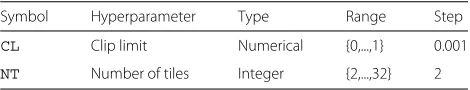
Therefore, to create an adequate labeled training set, we automatically extract a set of features from images and the expected CLAHE’s optimal hyperparameters. The process relied on generating contrast distorted images from ideal contrast ones. We defined a grid with CLAHE’s hyperparameters CL and NT, and for each original image, we evaluated each single combination of (CL, NT). The CLAHE’s hyper-space considered in experiments is pre-sented in Table1. The selected values for CL range from [ 0, 1] increased by a step of 0.001. For NT, the range is between {2, 32} with a step= 2. Thus, each image was evaluated by 1001×16 = 16016 different hyperparam-eter settings. The pair of hyperparamhyperparam-eters whose output image was the most similar to the original one was defined as thetargetvalue.

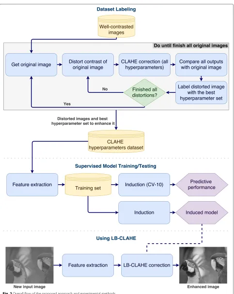
The overall flow of the proposed approach and exper-imental methods, showing the dataset labeling process, supervised model building, and validation steps, and the LB-CLAHE usage, can be seen in Fig.2. It is important to highlight that the final application of the proposed approach depends on just the induced model. In other words, a given new image is adjusted using the hyper-parameters predicted from the previously built model, induced only once.

The experimental methods adopted in this paper are presented in the following subsections. All the datasets and source code developed are freely available1.

Table 1Hyper-space considered in our experiments

Symbol Hyperparameter Type Range Step

CL Clip limit Numerical {0,...,1} 0.001

NT Number of tiles Integer {2,...,32} 2

2.1 Image datasets specification

Two image datasets were used in our experiments. The first one, dataset 1, was composed by 246 contrast distorted images from 54 ones. We merged two well-known image quality assessment (IQA) datasets to build thedataset 1: CSIQ [36] and TID2013 [37]. We gener-ated thedataset 1with the most popular IQA datasets in order to evaluate our method in different scenarios with quality distortions. Also, CSIQ and TID datasets were used in several recent contrast-related works [5,38,39].

In order to improve the generalizability of the proposed approach, and also to validate if it is facing more chal-lenging scenes and distortions, we created another dataset (dataset 2). In this new version, different from before, we created distortions to every ideal image provided in following IQA datasets: [40–46]. For each one of the 149 ideal images available, we created a set of 42 distor-tions. Thus,dataset 2was composed by 6258 contrast distorted images.

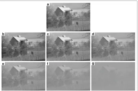
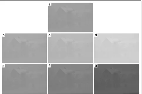
The set of 42 distortions was built using contrast and intensity variations. Each original image, considered as ideal by literature, had its contrast changed by histogram compression in six levels: {−50%, 10%, 30%, 50%, 70%, 90%}. Furthermore, the mean intensity of every changed level was also shifted in six histogram bins: {10, 30, 60} for both left and right sides. In Fig.3, all the contrast distor-tions from a given original image (without intensity shift) may be seen, while Fig.4depicts all intensity shifts of a contrast distorted image.

The histogram compression procedure, used to build the contrast distorted images, started by identifying the range of image intensities, in other words, by the extrac-tion of a distance between the leftmost and the right-most histogram bin. Then, this distance was decreased or increased to generate contrast distortions. We employed a linear distribution to obtain new values of left, right, and middle points for the compressed histogram. The Open Source Computer Vision Library (OpenCV)2was used to implement all distortions ofdataset 2images.

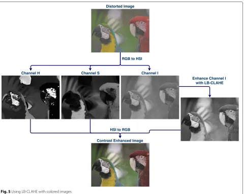
It is important to mention that, despite we used only the intensity (grayscale) channel from hue, saturation, and intensity (HSI) color space in our experiments, LB-CLAHE can also be applied to colored red, green, and blue (RGB) color space images. In this case, intensity chan-nel must be, along with the original hue and saturation channels, converted back to RGB after enhancement. This process can be seen in Fig.5.

2.2 Dataset labeling

a

b

c

d

e

f

g

Fig. 3Contrast distortions in dataset 2. Original image (a),₋50% compression (b), 10% compression (c), 30% compression (d), 50% compression (e), 70% compression (f), 90% compression (g)

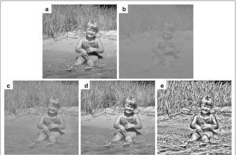
compared with the original image, searching for the most similar image pair. In other words, we tried all possible hyperparameter settings to correct those distorted ver-sions using the original image as the reference to find the best pair of h = {CL, NT}. Figure6depicts the impact of the hyperparameter values chosen to a given distorted image, with (a) being the original/ideal, (b) being the dis-torted one, and (c–e) being CLAHE outputs. Contrast was increased less than desired in (c), optimally increased in (d), and over increased in (e). It shows that it is important to select adequate CLAHE hyperparameters for a given image.

This process is analog to image similarity analysis, which can be performed by different aspects. In this work, the most important one was the similarity related to the image quality, especially regarding the contrast. The IQA tech-niques, which match this objective, can be split into three groups: (i) full reference, (ii) reduced reference, and with (iii) no reference [38, 47]. In a scenario where a refer-ence image is available to be compared to another, the full-reference techniques are preferred [38]. Therefore, we used three common IQA full-reference evaluation mea-sures: mean squared error (MSE), peak signal-to-noise

ratio (PSNR), and the structural similarity index (SSIM) index [47,48].

It is known that the entropy value (a statistical mea-sure of randomness) of a gray-level image is quite related with its contrast [26,38,49]. Thus, the entropy difference between both images (corrected and original) may be use-ful to identify images with similar contrast [49]. Here, we called it gray level entropy difference (GLED).

The MSE, PSNR, SSIM and GLED performance mea-sures present values from different ranges and scales. To create a trustful method to compute an indication from the metrics, we ordered the four metrics through calcu-lating an average rank. Thus, the highest ranked sample represents the most similar CLAHE/ideal image pair of hyperparameters.

The automatic labeling process is computationally expensive. A computer cluster composed of 18 computers (Intel Xeon E5-2430v2 and 24 GB RAM), with Windows 7 and Matlab, was used for this purpose.

2.3 Image features

a

b

c

d

e

f

g

Fig. 4Intensity shifts of histogram bins in dataset 2. Contrast distorted image with 90% compression (a), 10 bins to right (b), 30 bins to right (c), 60 bins to right (d), 10 bins to left (e), 30 bins to left (f), 60 bins to left (g)

to be described. Thus, the ML algorithms may be used to build models from the relations between image features and their labels.

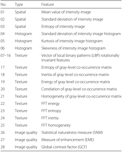
The features from images already provide useful infor-mation for automatic classification and regression [50]. In our proposal, we explore a set of 28 features to pre-dict effectively CL and NT values. These features may be divided into four main sub-groups: spatial, histogram, texture, and image quality.

As spatial image features (i.e., features extracted from each(x,y)pixel of the 2D image), two statistical moments (mean and standard deviation) and gray level entropy were selected. Based on the image histogram (tonal distribu-tion of a digital image), we extracted the second (standard deviation), third (skewness), and fourth (kurtosis) statisti-cal moments as suggested in [3,51].

Image texture features provide information about the spatial arrangement of intensities in an image. They have been applied in a wide variety of image classification appli-cations [52]. We used three common texture descriptors: local binary patterns (LBP) [53], gray-level co-occurrence matrix (GLCM) [52], and fast fourier transform (FFT) frequency domain features [50,54].

Fig. 5Using LB-CLAHE with colored images

O(N)[55–57]. Therefore, the time complexity for extract-ing image features is asymptotically dominated by the FFT calculation, i.e., our feature extraction step has time com-plexity ofO(NPlogP), considering thatNimages with the same spatial resolution are going to be processed.

2.4 Supervised regression algorithms

We evaluated a total of five different regression algorithms to determine which one would get the best performance in automatic CLAHE’s hyperparameter prediction. The choice was based on their extensive application in multi-ple predictive tasks, and also presenting different learning biases. In this way, the following algorithms were per-formed in our experiments: classification and regression tree (CART) [59], multilayer perceptron (MLP) artificial neural network [60], support vector machine (SVM) [61], random forest (RF) [62], and Extreme Gradient Boost-ing (XGBoost) [63]. All the regression techniques were performed using their standard hyperparameter settings,

as defined in the correspondingRpackages. The follow-ing sections briefly describe each one of the evaluated regression techniques.

2.4.1 CART

a

b

c

d

e

Fig. 6Automatic labeling process to find best CLAHE hyperparameter pair. Original image (a). distorted image (b). CLAHE with inacurrate hyperparameters: CL₌0.01 and NT₌[ 8, 8] (c). CLAHE with ideal hyperparameters: CL₌0.025 and NT₌[ 4, 4] (d). CLAHE with inacurrate hyperparameters: CL₌0.468 and NT₌[ 16, 16] (e)

2.4.2 MLP

Multilayer perceptron (MLP) feed-forward network [60] is an important class of artificial neural networks able to deal with classification and regression problems. MLPs are composed of multiple units (neurons), responsible for computing and propagating information through the net-work. These neurons are organized in layers, usually an input layer (which just receives the input values), one (or more) hidden layer(s), and an output layer. The informa-tion is propagated through the network feed-forwardly until the output layer. The back-propagation algorithm is often used to train the MLP networks. MLPs have been used to solve complex and diverse problems due to the generality of their application [60]. The RRSNNSpackage [66] was applied in our experiments.

2.4.3 SVM

Support vector machines (SVMs) [61] are kernel-based algorithms that performs non-linear classifica-tion/regression using a hyperspace transformation: it maps the inputs into a high-dimensional feature space

where the problem is linearly separable. SVMs are known to be robust in handling a wide variety of problems, presenting high accuracy and capacity to treat high-dimensional data. In this work, SVM implementation from thee1071R package [67] was used.

2.4.4 RF

Table 2List of all image features extracted

No. Type Feature

01 Spatial Mean value of intensity image

02 Spatial Standard deviation of intensity image

03 Spatial Entropy of intensity image

04 Histogram Standard deviation of intensity image histogram

05 Histogram Kurtosis of intensity image histogram

06 Histogram Skewness of intensity image histogram

07–16 Texture Vector of local binary patterns (LBP) rotationally invariant features

17 Texture Entropy of gray-level co-occurrence matrix

18 Texture Inertia of gray-level co-occurrence matrix

19 Texture Energy of gray-level co-occurrence matrix

20 Texture Correlation of gray-level co-occurrence matrix

21 Texture Homogeneity of gray-level co-occurrence matrix

22 Texture FFT energy

23 Texture FFT entropy

24 Texture FFT inertia

25 Texture FFT homogeneity

26 Image quality Statistical naturalness measure (SNM)

27 Image quality Measure of enhancement (EME)

28 Image quality Global contrast factor (GCF)

2.4.5 XGBoost

Extreme Gradient Boosting (XGBoost) [63] is a scal-able end-to-end tree ensemble boosting machine learning system based on the gradient boosting machine (GBM) framework that has provided state-of-the-art results on many problems. Sequentially, new trees are added to the ensemble aiming to minimize the actual error gradient (boosting) along a regularization term to avoid overfitting. In fact, XGBoost was reported as the best prediction tech-nique in several data mining competitions. We performed our experiments using theXGBoostR package.

2.5 Evaluation measures

For model assessment, we used the root mean square error (RMSE) and the determination coefficientR2 eval-uation measures. The RMSE was computed with the ideal CLAHE’s hyperparameters determined through the dataset and the predicted values by the regression model. This metric is defined as the root of the quadratic dif-ference between the true observed (yi) values and the

obtained (ˆyi) ones for each sample i of the n evaluated

cases [68], as defined by Eq.1. In our case, theyandyˆ val-ues represented, respectively, the desired CLAHE param-eters and its estimations made by the machine learning models. It measures how near of the expected values are the predictions made by the induced model.

RMSE= 1 n n

i=1

(yi− ˆyi)2. (1)

Ther-squared orR2expresses the amount of the total variation associated with the use of an independent vari-able. Its values range from 0 to 1: the closerR2is to 1, the higher is the proportion of the total variation in the output which is explained by introducing an independent variable in the regression scheme [69]. In this way,R2_{shows how}

similar are the predicted values when compared with the real expected, in our case, the CLAHE’s hyperparameters. All these information regarding the experimental setup is also presented in Table3.

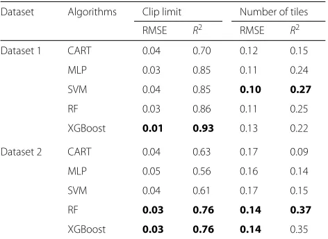
For dataset 1, regarding CL, best results were achieved by XGBoost, followed by RF. Still, best results while predicting the NT hyperparameter were achieved by SVM, closely followed by RF. For dataset 2, RF obtained the best results to both hyperparameters, fol-lowed by XGBoost. It is possible to observe that, in gen-eral, better results were observed in ensemble methods. Worst results were reached by MLP, probably because it relies on its tuning to achieve better results.

Table 3Experimental setup

Element Choice

Datasets Dataset 1: 246 contrast distorted images

Dataset 2: 6258 contrast distorted images

Full-reference IQA techniques

Mean squared error (MSE)

Peak signal-to-noise ratio (PSNR)

Structural similarity (SSIM)

Gray-level entropy difference (GLED)

Absolute mean brightness error (AMBE)

Visual information fidelity (VIF)

Image features Spatial (3 features)

Histogram (3 features)

Texture (19 features)

Image quality (3 features)

Supervised regression algorithms

Classification and regression tree (CART)

Multi-layer perceptron (MLP)

Support vector machine (SVM)

Random forest (RF)

Extreme Gradient Boosting (XGBoost)

Evaluation measures Root mean square error (RMSE)

R-squared (R2₎

Overall predictive performance was not high while pre-dicting NT. It is justified since image quality mainly depends on the CL rather than NT [26]. Thus, different NT values are capable to provide adequate images.

The RMSE supports the comparison of possible method superiority through the application of the Friedman’s sta-tistical test with significance level atα = 0.05. The null hypothesis is based on the equivalent performances of the algorithms considering the averaged RMSE on each dataset. Looking for emphasizing a possible superiority of an algorithm, we applied the Friedman’s statistical test, but was not observed significantly different between them (at p value = 0.1712). To select an algorithm to sup-port the discussions related to image features and contrast enhancement, we chose RF due to best position in Fried-man’s rank and capability of understanding the model by RF importance.

In this sense, the time complexity to build prediction models for the CLAHE hyperparameters would be related to the RF training cost. Non-prunned versions of tradi-tional decision tree algorithms, such as CART, present time complexity ofO(vNlogN), wherevrepresents the number of explaining features andNthe number of train-ing examples [59]. CART models are employed to com-pose the RF tree ensemble. Nonetheless, at each split point of thet trees in the forest, only sfeatures are explored, being the last ones selected at random. ThetandsRF’s hyperparameters are input by the user. Thus, the time complexity of training a RF predictor isO(tsNlogN). In our solution, RF is trained twice, corresponding to each of the CLAHE hyperparameters. Therefore, the compu-tational costs of our solution are the combination of the computations to extract the image features and to induce the regression models. Thus, the total asymptotic time complexity of our proposal isO(NPlogP+2tsNlogN), when consideringNimages with the same spatial resolution. The experiments were performed using the 10-fold cross-validation strategy owing to support a fair compari-son without overfitting.

3 Results and discussion

In this section, we present our main experimental results and findings. First, we present the results regarding the predictive performance of models from different ML algorithms. Afterwards, based on the best model performance, some results are discussed in the image enhancement context. Finally, a visual comparison of our method with [26] was performed.

3.1 Predictive performance

Table4 presents results regarding the predictive perfor-mance of the induced models for dataset 1 and for dataset 2. There, we present RMSE and R2 values achieved by the selected ML algorithms.

Table 4Predictive performance of machine learning regression algorithms fordataset 1anddataset 2

Dataset Algorithms Clip limit Number of tiles

RMSE R2 _{RMSE R}2

Dataset 1 CART 0.04 0.70 0.12 0.15

MLP 0.03 0.85 0.11 0.24

SVM 0.04 0.85 0.10 0.27

RF 0.03 0.86 0.11 0.25

XGBoost 0.01 0.93 0.13 0.22

Dataset 2 CART 0.04 0.63 0.17 0.09

MLP 0.05 0.56 0.16 0.14

SVM 0.04 0.61 0.17 0.15

RF 0.03 0.76 0.14 0.37

XGBoost 0.03 0.76 0.14 0.35

Best performances are highlighted

3.2 Image features importance

When using RF, by permuting the values of a feature in OOB samples and recalculating the OOBE in the whole ensemble, it is possible to address the RF variable impor-tance on prediction error. In other words, in the case of substituting the values of a particular feature by random values result in error boost, the feature is related to the positive problem comprehension. On the other hand, if the resulting importance is negative, the evaluated feature disrupts the task description and should be removed from modeling. This procedure could be performed for each feature toward explaining its impact [62].

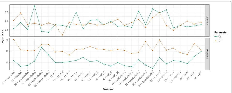
We used the RF importance to investigate the contribu-tion of each image feature in explaining the best CLAHE’s hyperparameter settings. In Fig.7, RF variable importance of each feature is presented. In the case of no nega-tive importance was obtained, no disrupted feature was selected in to build the model.

For CL, statistical moments of intensity image his-togram (features 4–6) were important. It is interesting to note that feature 4 was important only to dataset 1 while features 5 and 6 were more important todataset 2. Other features like 19 (energy of gray-level co-occurrence matrix), 22 (FFT energy), and 23 (FFT entropy) were also important to both datasets. Despite the importance peak of feature 10 indataset 1, LBP features achieved average importance values while predicting the CL hyper-parameter. Different than expected, two of the entropy-based features did not achieve high importance values: 3 (entropy of intensity) and 17 (entropy of gray-level co-occurrence matrix).

Fig. 7Features importance extracted from RF models, to both datasets and CLAHE hyperparameters

(standard deviation of intensity image), suggesting that a good NT value may have some correlation with image intensity.

Overall, no feature was useless at all. To have a faster feature extraction process, removing the less important features only may not be profitable. A better option is to perform group-based feature selection, once the removal of a complete group may have a higher impact on time during feature extraction.

3.3 Full-reference image quality assessment

In addition to the four IQA techniques used in the dataset labeling step, two more were used to eval-uate the similarity between the ideal (original) and obtained (contrast enhanced) images: absolute mean brightness error (AMBE) [70] and visual informa-tion fidelity (VIF) [71]. According to [72], most of the existing contrast enhancement evaluation mea-sures are not related to human perception of enhance-ment quality. Thus, we selected AMBE and VIF due to being full-reference techniques and exhibiting pos-itive correlations with perceptual quality of contrast enhancement.

Moreover, for comparison purposes, we used two base-lines: (i) CLAHE-fixed hyperparameters and (ii) global histogram equalization (HE). We fixed the CLAHE hyper-parameters as CL=0.01 and NT=[ 8, 8] (default of Matlab and others). Results of this comparison, for dataset 1, can be seen in Fig. 8. Regarding GLED, MSE, and AMBE, where lower values are desired, it is visible that LB-CLAHE achieved better results in most cases. On the other hand, regarding PSNR, SSIM, and VIF, higher val-ues are desired. Likewise, LB-CLAHE achieved noticeably better results in most cases.

Results were similar in dataset 2. As will be dis-cussed further in this section, there were a small set of images which LB-CLAHE was not superior. However, considering average values, LB-CLAHE achieved superior performance than the baselines to all the six IQA tech-niques experimented in both datasets. These values can be seen in Table5. In general, there were no significant dis-crepancy between the six IQA techniques regarding the performance of the three compared methods.

Figure 9 shows samples obtained by LB-CLAHE with high similarity considering the original image according to the IQA techniques for different contrast scenarios. It can be observed that in scenarios of adequate con-trast or more than enough (D), LB-CLAHE simply do not increase it. On the other hand, it properly enhances an image with low contrast (A, B, and C), giving it a natural aspect. Meanwhile, global HE and fixed CLAHE over-enhanced or under-enhanced the images in the four observed scenarios.

Table 5Average similarity values fordataset 1and

dataset 2

Dataset Method SSIM PSNR VIF MSE GLED AMBE

Dataset 1 Global HE 0.73 16.73 0.73 2046.12 1.76 26.65

Fixed CLAHE 0.78 18.36 0.84 1075.52 0.50 12.35

LB-CLAHE 0.90 23.39 0.89 396.26 0.22 8.78

Dataset 2 Global HE 0.75 16.51 0.69 2277.92 2.00 28.60

Fixed CLAHE 0.77 16.48 0.74 1949.75 0.60 25.56

LB-CLAHE 0.86 19.83 0.82 1181.10 0.17 20.91

Higher values are desired for SSIM, PSNR,and VIF. Lower values are desired for MSE, GLED, and AMBE

Best performances are highlighted

3.4 Visual comparison

We applied our method to the same set of images proposed by [26]. Although a full-reference com-parison is not possible due to irreproducibility of their work, we could observe in Fig. 11 that

both methods achieved similar visual results to all images.

Notwithstanding, the authors proposed a computation-ally costly task toward executing CLAHE with all pos-sible hyperparameter combinations to reach the result for a single image. Different from [26], our method extracts the image features to predict the hyperpa-rameters and perform CLAHE once. Also, we proved our method’s ability to enhance thousands of images over different contrast and illumination scenarios, while the method mentioned above was not extensively tested.

4 Conclusions

In this paper, we proposed the LB-CLAHE: a learning-based hyperparameter selection method for CLAHE using image features. We investigated the performance of our proposal with some well-known image sets and by the use of a huge distorted contrast image dataset. Several

a1 a2 a3 a4 a5

b1 b2 b3 b4 b5

c1 c2 c3 c4 c5

d1 d2 d3 d4 d5

a1 a2 a3 a4 a5

b1 b2 b3 b4 b5

c1 c2 c3 c4 c5

d1 d2 d3 d4 d5

Fig. 10LB-CLAHE’s low performance according to the IQA techniques. Best results achieved by global HE (A) and (B). Best results achieved by fixed CLAHE (C) and (D). Ideal image (1), distorted image (2), global HE (3), fixed CLAHE with CL₌0.01 and NT₌[ 8, 8] (4), proposed LB-CLAHE (5)

supervised regression algorithms were compared to build a suitable performance model. The best results were achieved by ensemble-based models induced with RF and XGBoost algorithm. Analysing the impact of each image feature in hyperparameter prediction, the RF impor-tance showed that no feature significantly stood out from the others. The experimental result confirmed that LB-CLAHE, a learning-based hyperparameter selection method for CLAHE, achieved superior performance in comparison to the histogram equalization and CLAHE with fixed and standard hyperparameters. Our method was capable of adjusting the images from different sce-narios, contrast, and illumination distortions. Further-more, once the model was created, it can be applied to quickly suggest the CLAHE’s hyperparameters for a

new image with superior performance over the compared methods.

4.1 Limitations and future works

a

b

c

Fig. 11Visual comparison between the entropy-based method proposed in [26] and LB-CLAHE. Office1 image(a), aerial image(b), announce image(c)

Endnotes

1_{http://www.uel.br/grupo-pesquisa/remid/?page_id=145}

2_{http://www.opencv.org}

Abbreviations

AMBE: Absolute mean brightness error; CART: Classification and regression tree; CL: Clip limit; CLAHE: Contrast Limited Adaptive Histogram Equalization; DT: Decision tree; EME: Measurement of enhancement by entropy; FFT: Fast fourier transform; GBM: Gradient boosting machine; GCF: Global contrast factor; GLCM: Gray-level co-occurrence matrix; GLED: Gray-level entropy difference; HDTV: High-definition television; HE: Histogram equalization; HSI: Hue, saturation, and intensity; IQA: Image quality assessment; LB-CLAHE: Learning-based contrast limited adaptive histogram equalization; LBP: Local binary patterns; ML: Machine learning; MLP: Multilayer perceptron; MSE: Mean squared error; NT: Number of tiles; OOB: Out-of-bag; OOBE: Out-of-bag error; OpenCV: Open source computer vision library; PSNR: Peak signal-to-noise ratio; RF: Random forest; RGB: Red, green, and blue; RMSE: Root mean square error; SNM: Statistical naturalness measure; SSIM: Structural similarity index;

SVM: Support vector machine; VIF: Visual information fidelity; XGBoost: Extreme Gradient Boosting

Acknowledgements

The authors would like to thank the Scientific Computing Lab at Londrina State University and Professor Taufik Abrão for providing the computer cluster which made this work possible, and to the grant #2012/23114-9 from São Paulo Research Foundation (FAPESP).

Funding

Not applicable.

Availability of data and materials

All the data supporting our findings, including datasets and source code developed, are freely available inhttp://www.uel.br/grupo-pesquisa/remid/? page_id=145.

Authors’ contributions

Authors’ information

Not applicable.

Competing interests

The authors declare that they have no competing interests.

Publisher’s Note

Springer Nature remains neutral with regard to jurisdictional claims in published maps and institutional affiliations.

Author details

1_{Electrical Engineering Department, Londrina State University, Rodovia Celso}

Garcia Cid, Londrina 86057-970, Brazil.2_{Computer Science Department,}

Londrina State University, Rodovia Celso Garcia Cid, Londrina 86057-970, Brazil.

3_{Institute of Mathematical and Computer Science (ICMC), University of São}

Paulo (USP), Av. Trabalhador São Carlense, 400, São Carlos 13566-590, Brazil.

4_{Computer Engineering Department, The Federal University of Technology}

-Paraná, Apucarana, Brazil.

Received: 21 September 2017 Accepted: 15 February 2019

References

1. M. H. Asmare, V. S. Asirvadam, A. F. M. Hani, Image enhancement based on contourlet transform. SIViP.9(7), 1679–1690 (2015)

2. H. Hiary, R. Zaghloul, A. Al-Adwan, M. B. Al-Zoubi, Image contrast enhancement using geometric mean filter. SIViP.11, 833–840 (2016) 3. R. C. Gonzalez, R. E. Woods,Digital image processing. (Pearson/Prentice

Hall, Upper Saddle River, 2008)

4. T. V. H. Laksmi, T. Madhu, K. C. S. Kavya, S. E. Basha, Novel image enhancement technique using CLAHE and wavelet transforms. Int. J. Sci. Eng. Technol.5(11), 507–511 (2016)

5. A. Saleem, A. Beghdadi, B. Boashash, Image fusion-based contrast enhancement. EURASIP J. Image. Video Process.2012(1), 1–17 (2012) 6. S. Gupta, Y. Kaur, Review of different local and global contrast

enhancement techniques for a digital image. Int. J. Comput. Appl.

100(18), 18–23 (2014)

7. A. M. Reza, Realization of the contrast limited adaptive histogram equalization (CLAHE) for real-time image enhancement. J. VLSI Signal Process. Syst. Signal Image Video Technol.38(1), 35–44 (2004) 8. K. Zuiderveld, inGraphics Gems IV, ed. by P. S. Heckbert. Contrast limited

adaptive histogram equalization (Academic Press Professional, Inc., San Diego, 1994), pp. 474–485

9. M. Sundaram, K. Ramar, N. Arumugam, G. Prabin, Histogram modified local contrast enhancement for mammogram images. Appl. Soft Comput.11(8), 5809–5816 (2011)

10. S. E. Kim, J. J. Jeon, I. K. Eom, Image contrast enhancement using entropy scaling in wavelet domain. Signal Proc.127, 1–11 (2016)

11. K. Akila, L. S. Jayashree, A. Vasuki, Mammographic image enhancement using indirect contrast enhancement techniques – a comparative study. Procedia Comput. Sci.47, 255–261 (2015). Graph Algorithms, High Performance Implementations and Its Applications (ICGHIA 2014) 12. W. G. Flores, W. C. de Albuquerque Pereira, A contrast enhancement

method for improving the segmentation of breast lesions on ultrasonography. Comput. Biol. Med.80, 14–23 (2017)

13. Y. M. George, B. M. Bagoury, H. H. Zayed, M. I. Roushdy, Automated cell nuclei segmentation for breast fine needle aspiration cytology. Signal Proc.93(10), 2804–2816 (2013). Signal and Image Processing Techniques for Detection of Breast Diseases

14. A. Tareef, Y. Song, W. Cai, H. Huang, H. Chang, Y. Wang, M. Fulham, D. Feng, M. Chen, Automatic segmentation of overlapping cervical smear cells based on local distinctive features and guided shape deformation. Neurocomputing.221, 94–107 (2017)

15. N. P. Singh, R. Srivastava, Retinal blood vessels segmentation by using Gumbel probability distribution function based matched filter. Comput. Methods Prog. Biomed.129, 40–50 (2016)

16. S. Aslani, H. Sarnel, A new supervised retinal vessel segmentation method based on robust hybrid features. Biomed. Signal Process. Control.30, 1–12 (2016)

17. N. R. S. Parveen, M. M. Sathik, in2009 International Conference on Computer Technology and Development, vol. 2. Enhancement of bone fracture images by equalization methods, (2009), pp. 391–394

18. L. Zheng, H. Shi, S. Sun, in2016 IEEE International Conference on Information and Automation (ICIA). Underwater image enhancement algorithm based on CLAHE and USM, (2016), pp. 585–590 19. X. Qiao, J. Bao, H. Zhang, L. Zeng, D. Li, Underwater image quality

enhancement of sea cucumbers based on improved histogram equalization and wavelet transform. Inf. Process. Agric.4, 206–213 (2017) 20. E. A. Murillo-Bracamontes, M. E. Martinez-Rosas, M. M. Miranda-Velasco,

H. L. Martinez-Reyes, J. R. Martinez-Sandoval, H. Cervantes-de-Avila, Implementation of Hough transform for fruit image segmentation. Procedia Eng.35, 230–239 (2012). International Meeting of Electrical Engineering Research 2012

21. W. Ji, Z. Qian, B. Xu, Y. Tao, D. Zhao, S. Ding, Apple tree branch segmentation from images with small gray-level difference for agricultural harvesting robot. Optik - Int. J. Light Electron Opt.127(23), 11173–11182 (2016)

22. L. Unzueta, M. Nieto, A. Cortes, J. Barandiaran, O. Otaegui, P. Sanchez, Adaptive multicue background subtraction for robust vehicle counting and classification. IEEE Trans. Intell. Transp. Syst.13(2), 527–540 (2012) 23. A. Gudigar, S. Chokkadi, U. Raghavendra, U. R. Acharya, Local texture

patterns for traffic sign recognition using higher order spectra. Pattern Recogn. Lett.94, 202–210 (2017)

24. X. Wang, X. Liu, H. Guo, Q. Guo, N. Liu, Research on pedestrian detection method with motion and shape features. J. Comput. Theor. Nanosci.

13(9), 5788–5793 (2016)

25. L. G. Moré, M. A. Brizuela, H. L. Ayala, D. P. Pinto-Roa, J. L. V. Noguera, in 2015 IEEE International Conference on Image Processing (ICIP). Parameter tuning of CLAHE based on multi-objective optimization to achieve different contrast levels in medical images, (2015), pp. 4644–4648 26. B. S. Min, D. K. Lim, S. J. Kim, J. H. Lee, A novel method of determining

parameters of CLAHE based on image entropy. Int. J. Softw. Eng. Appl.

7(5), 113–120 (2013)

27. H. Hiary, R. Zaghloul, A. Al-Adwan, M. B. Al-Zoubi, Image contrast enhancement using geometric mean filter. SIViP.11(5), 833–840 (2017) 28. M. Sepasian, W. Balachandran, C. Mares, inProceedings of the World

Congress on Engineering and Computer Science. Image enhancement for fingerprint minutiae-based algorithms using CLAHE, standard deviation analysis and sliding neighborhood, (2008), pp. 22–24

29. A. łoza, D. R. Bull, P. R. Hill, A. M. Achim, Automatic contrast enhancement of low-light images based on local statistics of wavelet coefficients. Digit. Signal Proc.23(6), 1856–1866 (2013)

30. N. M. Sasi, V. Jayasree, Contrast limited adaptive histogram equalization for qualitative enhancement of myocardial perfusion images. Engineering.5, 326 (2013)

31. P. Li, L. Dong, H. Xiao, M. Xu, A cloud image detection method based on SVM vector machine. Neurocomputing.169, 34–42 (2015). Learning for Visual Semantic Understanding in Big Data ESANN 2014 Industrial Data Processing and Analysis

32. M. Quintana, J. Torres, J. M. Menéndez, A simplified computer vision system for road surface inspection and maintenance. IEEE Trans. Intell. Transp. Syst.17(3), 608–619 (2016)

33. S. U. Sharma, D. J. Shah, A practical animal detection and collision avoidance system using computer vision technique. IEEE Access.5, 347–358 (2017)

34. T. M. Mitchell,Machine learning. (McGraw Hill, New York, 1997) 35. Y. Yao, J. Zhang, F. Shen, X. Hua, J. Xu, Z. Tang, A new web-supervised

method for image dataset constructions. Neurocomputing.236, 23–31 (2017)

36. E. C. Larson, D. M. Chandler, Most apparent distortion: full-reference image quality assessment and the role of strategy. J. Electron. Imaging.

19(1), 011006–011006 (2010)

37. N. Ponomarenko, O. Ieremeiev, V. Lukin, K. Egiazarian, L. Jin, J. Astola, B. Vozel, K. Chehdi, M. Carli, F. Battisti, et al., inVisual Information Processing (EUVIP), 2013 4th European Workshop On. Color image database tid2013: Peculiarities and preliminary results (IEEE, 2013), pp. 106–111 38. A. Shokrollahi, A. Mahmoudi-Aznaveh, M.-N. B.Maybodi, Image quality

assessment for contrast enhancement evaluation. AEU - Int. J. Electron. Commun.77, 61–66 (2017)

39. A. Saleem, A. Beghdadi, B. Boashash, A distortion-free contrast enhancement technique based on a perceptual fusion scheme. Neurocomputing.226, 161–167 (2017)

Za Automatiku, Mjerenje, Elektroniku, Raˇcunarstvo I Komunikacije.53(4), 344–354 (2012)

41. J. Y. Lin, S. Hu, H. Wang, P. Wang, I. Katsavounidis, A. Aaron, C. J. C-Kuo, Statistical study on perceived JPEG image quality via MCL-JCI dataset construction and analysis. Electron. Imaging.2016(13), 1–9 (2016) 42. S. Hu, H. Wang, C. J. C-Kuo, inAcoustics, Speech and Signal Processing

(ICASSP), 2016 IEEE International Conference On. A gmm-based stair quality model for human perceived jpeg images (IEEE, 2016), pp. 1070–1074 43. J. Y. Lin, L. Jin, S. Hu, I. Katsavounidis, Z. Li, A. Aaron, C. J. C.-Kuo, inSPIE

Optical Engineering+ Applications. Experimental design and analysis of jnd test on coded image/video (International Society for Optics and Photonics, 2015), pp. 95990–95990

44. P. Le Callet, F. Autrusseau, Subjective quality assessment IRCCyN/IVC database (2005).http://www2.irccyn.ecnantes.fr/ivcdb/

45. H. R. Sheikh, M. F. Sabir, A. C. Bovik, A statistical evaluation of recent full reference image quality assessment algorithms. IEEE Trans. Image Process.15(11), 3440–3451 (2006)

46. Z. Wang, A. C. Bovik, H. R. Sheikh, E. P. Simoncelli, Image quality assessment: from error visibility to structural similarity. IEEE Trans. Image Process.13(4), 600–612 (2004)

47. H.Y.V., H. Y. Patil, Article: A survey on image quality assessment techniques, challenges and databases. IJCA Proc. Natl. Conf. Adv. Comput.NCAC 2015(7), 34–38 (2015). Full text available

48. N. Thakur, S. Devi, A new method for color image quality assessment. Int. J. Comput. Appl.15(2), 10–17 (2011)

49. K. Gu, G. Zhai, W. Lin, M. Liu, The analysis of image contrast: From quality assessment to automatic enhancement. IEEE Trans. Cybern.46(1), 284–297 (2016)

50. M. S. Nixon, A. S. Aguado,Feature Extraction & Image Processing for Computer Vision. (Academic Press, Oxford, 2012)

51. D. Li, N. Li, J. Wang, T. Zhu, Pornographic images recognition based on spatial pyramid partition and multi-instance ensemble learning. Knowl.-Based Syst.84, 214–223 (2015)

52. R. M. Haralick, K. Shanmugam, I. Dinstein, Textural features for image classification. IEEE Trans. Syst. Man Cybern.SMC-3(6), 610–621 (1973) 53. T. Ojala, M. Pietikäinen, T. Mäenpää, Multiresolution gray-scale and

rotation invariant texture classification with local binary patterns. IEEE Trans. Pattern. Anal. Mach. Intell.24(7), 971–987 (2002)

54. H. Shen, P. Chen, L. Chang, Automated steel bridge coating rust defect recognition method based on color and texture feature. Autom. Constr.

31(0), 338–356 (2013)

55. H. Yeganeh, Z. Wang, Objective quality assessment of tone-mapped images. IEEE Trans. Image Process.22(2), 657–667 (2013)

56. S. S. Agaian, K. Panetta, A. M. Grigoryan, Transform-based image enhancement algorithms with performance measure. IEEE Trans. Image Process.10(3), 367–382 (2001)

57. K. Matkovi´c, L. Neumann, A. Neumann, T. Psik, W. Purgathofer, in Proceedings of the First Eurographics Conference on Computational Aesthetics in Graphics, Visualization and Imaging. Global contrast factor - a new approach to image contrast (Eurographics Association, Aire-la-Ville, 2005), pp. 159–167

58. O. A. Penatti, E. Valle, S. R.d.Torres, Comparative study of global color and texture descriptors for web image retrieval. J. Vis. Commun. Image Represent.23(2), 359–380 (2012)

59. L. Breiman, J. Friedman, C. J. Stone, R. A. Olshen,Classification and Regression Trees. (CRC press, New York, 1984)

60. S. Haykin, Neural network: a compressive foundation (1999)

61. V. N. Vapnik,The Nature of Statistical Learning Theory. (Springer, New York, 1995)

62. L. Breiman, Random forests. Mach. Learn.45(1), 5–32 (2001)

63. T. Chen, C. Guestrin, inProceedings of the 22Nd ACM SIGKDD International Conference on Knowledge Discovery and Data Mining. Xgboost: A scalable tree boosting system (ACM, New York, 2016), pp. 785–794

64. L. Rokach, O. Maimon,Data Mining With Decision Trees: Theory and Applications, 2nd edn. (World Scientific Publishing Co., Inc., River Edge, 2014)

65. T. Therneau, B. Atkinson, B. Ripley, Rpart: recursive partitioning and regression trees (2015). R package version 4.1-10.https://CRAN.R-project. org/package=rpart

66. C. Bergmeir, J. M. Benítez, Neural networks in R using the Stuttgart neural network simulator: RSNNS. J. Stat. Softw.46(7), 1–26 (2012)

67. D. Meyer, E. Dimitriadou, K. Hornik, A. Weingessel, F. Leisch, E1071: Misc Functions of the Department of Statistics, Probability Theory Group (Formerly: E1071), TU Wien (2017). R package version 1.6-8.https://CRAN. R-project.org/package=e1071

68. T. Chai, R. R. Draxler, Root mean square error (RMSE) or mean absolute error (mae)?. Geosci. Model Dev. Discuss.7, 1525–1534 (2014) 69. J. A. Cornell, R. D. Berger, Factors that influence the value of the

coefficient of determination in simple linear and nonlinear regression models. Phytopathology.77(1), 63–70 (1987)

70. S.-D. Chen, A. R. Ramli, Minimum mean brightness error bi-histogram equalization in contrast enhancement. IEEE Trans. Consum. Electron.

49(4), 1310–1319 (2003)

71. H. R. Sheikh, A. C. Bovik, Image information and visual quality. IEEE Trans. Image Process.15(2), 430–444 (2006)