Raghunath Arnab
Department of Statistics, University of Botswana and Department of Statistics, University of KwaZulu-Natal, South Africa
Email: [email protected]
George Anderson
Department of Computer Science, University of Botswana,Botswana Email: [email protected]
John. O. Olaomi
Department of Statistics, University of South Africa, South Africa Email: [email protected]
B. C. Rodríguez
Department of Statistics and Operations Research, Universidad de Granada, Spain Email: [email protected]
Abstract
We propose an alternative two-phase stratified ranked set sampling. A comparison of the performances of the proposed estimators made by simulation studies using both real and simulated data sets. It is found that the proposed two-phase stratified regression estimator beats its competitors in literature.
AMS Subject Classification: 62D05
Keywords: Order statistics, ranked set sampling, relative efficiency, sampling with replacement, two-phase sampling.
1. Introduction
Ranked set sampling (RSS) introduced by McIntyre (1952), was used to estimate the mean pasture and forage yield. The RSS is employed when precise measurement of the variable of interest is difficult or expensive, but one can easily rank the variable without measuring the variable by an inexpensive method such as visual perception, judgment and auxiliary information. For example, in the problem of estimating the mean height of trees in a forest, one can rank the heights of a small sample of two or three trees standing nearby easily by visual inspection without measuring them. In estimating the number of bacterial cells per unit volume, we can rearrange two or three test tubes easily in order of concentration using optical instruments without measuring exact values. In the RSS, instead of selecting a single sample of sizem, we select m- sets of samples each of sizem. In each set, we rank all the elements but we only measure one of them. Finally, the average of them- measured units is taken as an estimate of the population mean.
replacement (SRSWR) of the same size. Dell and Clutter (1972) proved that the sample mean based on the RSS is unbiased for the population mean regardless of the ranking error and it is at least as precise as the SRSWR sample mean of the same size. Stokes (1977) considered the performance of the Dell and Clutter estimator when the regression of the study variable (y) and the ranking variable (x) is linear, and y and x follow certain model. Yu and Lam (1997) proposed regression estimator when x and y follow a bivariate normal distribution and found on the basis of simulation studies that their proposed regression estimator performs better than the naive estimator, unless the correlation between x and y is low (|ρ|< 0.4). Kadilar et al., (2006) and Arnab and Olaomi (2015) proposed an improved estimator of mean y, the population mean of the study variable yusing the ranking variable as an auxiliary variable x when the population mean x of x is unknown. Zamanzade and Al-Omari (2016) developed a new ranked set sampling for estimating the population mean and variance, called neoteric ranked set sampling (NRSS) under perfect and imperfect ranking conditions while Mahdizadeh and Zamanzade (2018) introduced stratified pair ranked set sampling (SPRSS) and utilized it in estimating the population mean, with some theoretical results.
In this paper, we propose two alternative estimators for two-phase sampling where in the first phase; information only on the ranking variable x is collected. Based on the observed x - values, the population is divided into a number of homogeneous strata. From each of the stratum so formed, one selects ranked set samples independently using proportional allocation. The performances of the proposed estimators are compared by simulation studies using both real tree data collected by Platt et al. (1988) and generated bivariate normal data. We found that the proposed two-phase stratified regression estimator performs better in respect of relative bias (RB) and mean-square error (MSE) than those of naïve and Yu and Lam (1997) estimators for the tree data and it behaves better in most situations for the simulated bivariate data.
1.1. Rank set sampling by SRSWR method
First, we choose a small number m (set size) such that one can easily rank the m elements of the population with sufficient accuracy. Then the selection of RSS is as follows: Select a sample of 2
m units from a population U by SRSWR method. Allocate these 2
m units at random into msets each of sizem. Rank all the units in a set with respect to the values of the variable of interest y from 1(minimum) to m(maximum) by a very inexpensive method such as eye inspection. At this stage, no actual measurement is done. After the ranking has been completed, the unit holding rank i(i=1,..,m) in the ith set is actually measured. This completes a cycle of the sampling. One repeats the process for r cycles to obtain the desired sample of sizen=mr. Thus, in a RSS, a total of m r2 units are drawn from the population but only mrof them are measured and the rest mr m( −1)are discarded. We
call these measured mr observations “ranked set sample”. Since the ordering of a large number of observations is difficult, increase of sample size n=mris done by increasing the number of cycles r. It is well known that ˆ ( , )rss m r , the sample mean the RSS of size n=mr is unbiased for the population mean y.
1.2. Judgment ranking
such as visual inspection, expert opinion or use of concomitant variable. It should be noted that some tests have been developed in the literature to assess the assumption of perfect ranking in RSS. Some of these include Frey, et al (2007), Zamanzade, et al (2012) and Zamanzade and Vock (2018).
Let yi j k| be the smallest j th “judgment order statistic” corresponding to order statistic
( )| i j k
x of the concomitant variable x in the i th set of the cycle k. In case the judgment ranking is perfect yi j k| becomes equal to the jth order statisticyi j k( )| , otherwise if the judgment process is imperfect, we findyi j k| yi j k( )| .
Stokes (1977) derived the following results: Theorem 1.
(i) |
1 1 ˆ
r
rss m k
k y r
=
=
is an unbiased estimator for y.(ii) The variance of ˆrss is
( )
2 2
| 1
1 1
ˆ
m
y
rss j m
j V
n m
=
= −
(iii) An unbiased estimator of the variance of V
(
ˆrss)
is
( )
(
|)
21 1
ˆ ˆ ˆ
( 1)
r
rss m k rss
k
V y
r r
=
= −
−
1.3. Use of auxiliary variable with known meanx
Stokes (1977) considered the linear regression of yon x as follows:
y=y+B x( −x)+ (1)
where xand are independent random variables, E( | )x =0, V( | )x =2y(1−2), y x B
=
and is the correlation coefficient between xandy. The equation (1) yields
i i k| y
(
i i k( )| x)
i i k( )|y = +B x − + (2)
Stokes (1977) further assumed that y y y
−
and x
x x
−
have the same marginal distribution,
which holds for bivariate normal and bivariate Pareto distributions. Stokes (1977) derived the following Theorem:
Theorem 2. (i) E
(
ˆy rss)
=y(ii)
(
)
2
2 2
| 1 1
ˆ
m
y y j m
y rss
j V
mr m
=
= −
where |
1 1 1 ˆ
r m
j j k y rss
k j
y mr
= =
Following Stokes (1977), Yu and Lam (1997) proposed the following estimator of the population mean y of yas
ˆyreg =ˆy rss −Bˆ
(
ˆx rss( )−x)
(3)where
( ) ( )|
1 1 1 ˆ
r m
x rss j j r
k j
x mr
= =
=
and(
)(
)
(
)
| ( )| ( )
1 1
2 ( )| ( ) 1 1
ˆ ˆ
ˆ
ˆ r m
j j k y rss j j k x rss k j
r m
j j k x rss k j
y x
B
x
= =
= =
− −
=
−
(4)Yu and Lam (1997) derived the following theorem: Theorem 3.
(
ˆ)
( ) i E yreg =y
( )ii The optimum value of Bˆ that minimizes the variance of ˆyreg is B.
(
)
2(
2)
(2 )2 1
ˆ
( ) yreg y 1 rss
z Z
iii Var E
mr S
= − +
(
)
(
)
2
2 2
( ) 2
( ) 1
1
y rss x
x rss x E
mr s
− −
= +
where
( )| ( )
( ) ( )|
1 1 1 1
1 r m 1 r m j j k x rss x
rss j j k
x x
k j k j
x x
Z z
mr mr
= = = =
− −
=
=
=(
)
2 ( )| ( ) 22
( )| ( )
1 1 1 1
1 r m 1 r m j j k rss
z j j k rss
x
k j k j
x x
S z Z
mr = = mr = =
−
= − =
2 2( )/
x rss x
s
= and
(
)
22
( ) ( )| ( )
1 1
1 r m
x rss j j k rss
k j
s x x
mr = =
=
− .1.4. Population mean with unknownx
Since xis unknown, Yu and Lam (1997) considered a two-phase sampling procedure where in the first-phase, a relatively large sample sof size n is selected by the simple random sampling without replacement (SRSWOR) method from a population of size N and only information on the auxiliary variable x is collected. On the second-phase, a sub-sample s of size n(=rm) is selected from s using ranked set sampling with r cycles and information of study variable y is obtained using x as ranking variable. The proposed estimator for the population mean y is
ˆYM =ˆy rss −Bˆ
(
ˆx rss( )−x')
(5)where ' i/
i s
x x n
=
and Bˆ is defined in (4).Yu and Lam (1997) derived the following results for large N and assuming the model (2) holds.
Theorem 4.
(ˆ )
( ) i E YM =y
(
)
(
)
(
)
2
2 2 2 2
( )
2 1
ˆ
( ) YM y 1 rss y
z
Z Z
iii Var E
mr S n
− −
= + +
(
)
(
)
22 2 2 2
( )
2 ( )
1 '
1
y rss y
x rss
x x
E
mr s n
− −
= + +
(6)
where Z=(x'−x)/x , Z(rss) , x(rss), 2
Z
S and s2x rss( ) are defined as in Theorem 3.
2. Two-phase stratified ranked set sampling
Initially, a relatively large sample sof size n is selected from the entire population by SRSWOR method. From each of the selected units of s, information only on the concomitant variable x is obtained similar to Yu and Lam (1977) in two-phase sampling. Here, we assume that the condition of two-phase sampling is valid i.e. the cost of collecting data on xis much cheaper than that of the study variabley. Observing the values of x, the sampled units are classified into a number of strata Hso that each of the stratum becomes homogeneous with respect to the variable under study y. The number of strata will certainly depend on the characteristics of the variable y and sample size n. For example, noting eye estimates of heights or date of plantation, one can classify the plants as small, medium or big. Similarly, noting the CD counts of HIV patients, we may classify the conditions of the HIV infected patients into bad, very bad and severe. Let sh be the set of units of size nhfalling in the hth stratum. Here nh is a random variable taking values from 0 to min (nh,Nh)where Nh is the total number of the units in the hth stratum of the population. From the sampled nhunits of the hth stratum, a sub-sample of sh(sh) of size
h h h h
n = n =mr units is selected using a ranked-set sampling procedure with rhcycles of set-size m each using the x as ranking variable where h(0h 1)are pre-determined
fractions (vide Rao, 1973). Here we assume that (i) n is so large that P n( h1)=1 and (ii)
h
r are integers. For proportional allocation with fixed sample size h h
n n
=
, h = = n n/
and nh=n n nh / =mrh.
Let the ranked set data collected from the hstratum be denoted by
(
( ) ( ))
|h, ( )|h ; 1,.., ; 1,..,
h h
h j j t j j t h h
d = y x j= m t = r ; h=1,...,H (7)
where ( ) ( )|h
h j j t
x is the jth ordered statistics for the concomitant variable xof the jth set of
h
t th cycle of the hth stratum and ( ) |
h
h j j t
y be the corresponding judgment order statistic for the study variable fory.
2.1. Estimator of the population mean without using auxiliary variable at the estimation stage
1
ˆ ˆ
H
st h
yrss h y rss h w = =
(8)where h
h n w
n
= and ( ) |
1 1 1 ˆ h h h r m h h
y rss j j t
h t j
y mr = = =
. Theorem 5. (i) styrss
is an unbiased estimator of y
(ii)
( )
2 2 |(
)
21 1
1 1 1
ˆ
H m
st
yrss h hy h j m hy y
h h j V W n m = = = − + −
where hy and 2
hy
are the population mean and variance of y for the stratum h,
| |
h j m h j m hy
= − , |
(
|)
h
h h j m E yj j t
= and Whis the proportion of units in the population
of the hth stratum. Proof:
Since 𝑛̃ℎ, the number of units in 𝑛 that fall into hth stratum is a random variable, we have from Rao (1973)
h h
E w W , V wh Wh 1 Wh n ,
' '
, h h
h h
W W Cov w w
n ,
(
ˆ |)
hy rss h hy
E n = and
(
)
2 2 | 1 1 1 ˆ | m hy rss h hy h j m
h j V n n m = = −
(9)Using (9), we get the following:
(i)
(
)
(
)
1
ˆ ˆ |
H
st h
y rss h y rss h
h
E E w E n
=
=
1H
h hy h
E w
=
=
1H
h hy h
W
=
=
=y(ii)
(
)
2(
)
(
)
1 1
ˆ ˆ | ˆ |
H H
st h h
y rss h y rss h h y rss h
h h
V E w V n V w E n
= = = +
(10)Now using Theorem 1, we find
(
ˆhy rss | h)
hyE n = and
(
)
2 2 |1
1 1
ˆ |
m h
y rss h hy h j m
h j V n n m = = −
(11)The first component of (10) is obtained from (11) as
(
)
2 1 ˆ | H hh y rss h
h
E w V n
=
2 2 2 | 1 1 1 1 H m hhy h j m
h h
h j
n E
n n m
= = = −
(noting, nh =h hn )
2 2
|
1 1
1 H h 1 m
hy h j m
h
h j
W
n = m =
= −
(12)The second component of (10) is
(
)
1 1
ˆ |
H H
h
h yreg h h hy
h h
V w E n V w
= = =
( )
(
)
2 ' '1 ' 1
,
H H H
hy h hy h y h h
h h h
V w Cov w w
= =
=
+
(13)(
)
2 21 1 1
1
ˆ |
H H H
h
h yreg h h hy h hy
h h h
V w E n W W
n = = = = −
(
)
2 1 1 Hh hy y
h W
n =
= −
(14)Part II of the theorem follows from (10), (12) and (14). Corollary 1.
For proportional allocation with fixed sample size n at the second phase, V
(
ˆstyreg)
reduces to( )
(
)
22 2
|
1 1
1 1 1
ˆ
H m
st
yrss h hy h j m hy y
h j
V W
n m n
= = = − + −
2.2. Using auxiliary information at the estimation stage
Noting ( ) |
1 1 1 ˆ h h h k m h h
y rss j j t
h t j
y mr
= =
=
and ( ) ( )( )| ( )1 1 1 ˆ h h h k m h h
x rss j j t h rss
h t j
x x
mr
= =
=
= are unbiasedestimators of the population means hy and hx of yand xof the stratum hrespectively,
we propose the following regression estimator of the population mean y of yas
1
ˆ ˆ
H
st h
yreg h yreg h
w
=
=
where wh =nh/n, ˆh ˆh ˆh
(
ˆh( ) ')
yreg y rss B x rss xh = − − , ' 1
h
h i
h i s
x x n =
and(
)(
)
(
)
( ) ( ) | ( )| 1 1 2 ( ) ( )| 1 1 ˆ ˆ ˆ ˆ h h h h h h h r mh h h h
y rss x rss
j j t j j t
t j
h
r m
h h
x rss j j t
t j y x B x = = = = − − = −
Assume that h
( )
h i iy x , is the value of y x( )for the i th unit of theh( 1,...,= H)th stratum
follows the model.
(
)
h h h
i hy h i hx i
y = +B x − + (15)
where h i
x and ih are independent random variables; E x
( )
ih =hx, V x( )
ih =hx2, E y( )
ih =hy,;
( )
h 2i hy
V y == ; E(ih|xih)=0 , ( h| h) 2 (1 2)
i i hy h
V x = − , h h hy hx
B
= , and h is the correlation
coefficient between xandy of the hth stratum.
Theorem 6.
Under the model (15) (i) st
yreg
is an unbiased estimator of y
(ii)
(
)
(
)
(
)
(
)
2
2 2 2 2
2 2 1 1 1 1 1 ˆ 1
H hy h hrss h H
h hy st
yreg h h hy y
h hz h
h h
Z Z
V W E W
n S m n
(
)
(
)
2(
)
2 2 ' 2 2
2 ( ) 2 ( ) 1 1 1 1 1 1
H hy h h rss h H
h hy
h h hy y
h hx rss h
h h
x x
W E W
n s m n
= = − − = + + + −
where ( ) ( )|
1 1 1 rh m h
h rss j j k
h k j
Z z
mr = =
=
, 2(
( )| ( ))
21 1 1 rh m h
hz j j k h rss
h k j
S z Z
mr = =
=
− ,(
)
22
( ) ( )| ( )
1 1
1 rh m
h
hx rss j j k h rss
h k j
s x x
mr = =
=
− , ( )| ( )|h
j j k hx h
j j k
hx x z − = , ' h hx h hx x Z −
= and ' 1
h
h hi
h i s
x x
n
=
.Proof:
(i)
( )
(
)
1
ˆ ˆ |
H
st h
yreg h yreg h
h
E E w E n
=
=
1H
h hy h
E w
=
=
1H
h hy h
W
=
=
=y(ii)
( )
2(
)
(
)
1 1
ˆ ˆ | ˆ |
H H
st h h
yreg h yreg h h yreg h
h h
Var E w V s V w E s
= =
= +
(16)Now using (6), we find
(
)
2(
2)
(
)
2 2 22 2
1
ˆhyreg | h hy h 1 hrss h h hy
h hz h
Z Z
V s E
mr S r m
− − = + +
(
)
(
)
22 2 2 2 2
2 1
1
hy h hrss h h hy
h hz h
Z Z
E
n S mn
− − = + + (17)
Equation (17) yields the first component of (16) as
(
)
2 1 ˆ | H hh yreg h
h
E w V n
=
(
)
(
)
22 2 2 2
2 2 1 1 1 H
hy h hrss h h hy
h
h h hz h h
h
Z Z
n
E E
n n S m n
= − − = + +
(
)
(
)
22 2 2 2 2
2 1
1 1
1
H hy h hrss h
h hy h
h hz h
h
Z Z
W E
n S m
= − − = + +
(18)
(
)
(
)
22 2 2 2 2
2 1
1 1
1
H hy h hrss h
h hy h
h hz h
h
Z Z
W E
n S m
= − − = + +
The second component of (16) is obtained from (14) as
(
)
1 1
ˆ |
H H
h
h yreg h h hy
h h
V w E n V w
= = =
(
)
2 1 1 Hh hy y
h W
n =
= −
(19)Part II of the theorem follows from (16), (18) and (19).
Corollary 2.
(
)
(
)
(
)
2 2 2(
)
22 2
2
1 1
1 1
ˆ 1 1
H hrss h H
h hy st
yreg h hy h h hy y
hz
h h
Z Z
V W E W
n S m n
= =
−
= − + + + −
(
)
(
')
2 2 2(
)
2( )
2 2
2 ( )
1 1
1 1
1 1
H h rss h H
h hy
h hy h h hy y
hx rss
h h
x x
W E W
n s m n
= =
−
= − + + + −
where ( ) ( )| ( )| ( )
1 1 1 1
1 rh m 1 rh m h
j j k hx h rss hx
h
h rss j j k
h k j h k j hx hx
x x
Z z
mr mr
= = = =
− −
=
=
= and' '
( ) ( )
h rss hx h hx h rss h
hrss h
hx hx hx
x x x x
Z Z
− − −
− = − = .
3. Comparison of stratified and un-stratified ranked set sampling strategies
It is very difficult to compare the performances of the proposed estimators 2 ˆst yreg
t = and
3 ˆstyrss
t = theoretically with the existing estimators t0=ˆy rss (Stokes, 1977) and t1=ˆYM (Yu and Lam, 1997), since the expressions of the variances Var t( );j j=0,1, 2 involve several
unknown parameters. Hence, we will compare the performances using simulation studies. For the simulation studies, we have considered both real and simulated data.
The real tree data related to the diameter in centimetres at breast height (x) and entire height (y) in feet of 396 trees which was originally collected by Platt et al. (1988) and used later by Chen et al. (2003) and Zamanzade and Mahdizadeh (2018). The mean diameter and heights of 396 (=N) trees are x= 20.970 cm and y= 52.967 feet respectively. The tree were portioned into two strata with diameter less than equal 13.6 cm (stratum 1) and more than 13.6 cm (stratum 2) respectively.
The number of trees belonging to the stratum 1 and stratum 2 are equal to 198. In the first-phase, a sample s of size n is selected from the entire population by the SRSWOR method and information only on the auxiliary variable x is collected. Let si be the sample of size
i
n that falls in the stratumi( 1, 2)= . From the sample si, a sub-sample of size si of size
/
i i
n = nn n is collected using proportional allocation by RSS sampling with m(=2, 3, 4)as
set-size and n as a predetermined number. For our simulation studies we take the following combinations of (n n m, , ): (250,160,2), (250,160,3), (250,160,4); (250,100,2), (250,100,3),
(250,100,4); (200,125,2), (200,125,3), (200,125,4); (200,80,2), (150,80,3), (200,80,4); (150,80,2), (150,80,3), (150,80,4); (150,60,2), (150,60,3), (150,60,4).
The simulated data comprises with 5 bivariate normal populations of sizes 600 (=N) each
of which have the same x =10, y =25, x=2.5,y =4.5 but different values of
( 0.5, 0.6, 0.7, 0.8, 0.9)
= . We divide each population into two strata as the tree population.
From each of the 5 populations, ranked set samples of parameters (n n m, , ): (400,125,2),
(400,125,3), (400,125,4); (400,80,2), (400,80,3), (400,80,4); (250,80,2), (250,80,3), (250,80,4) are selected.
, t1 , t2 and t3 based on the qth iteration be denoted by t q0( ), t q1( ), t q2( ) and t q3( ) respectively. The relative biases (RB) and the mean square errors (MSE) of the estimators are computed using the following formula:
( )
1
1 1
( )
R
j j y
y q
RB t t q
R
=
= −
and
( )
(
)
21 1
( ) R
j j y
q
MSE t t q
R =
=
− ; j=0,1, 2, 3 (20)The percentage relative efficiency of the estimator tj compared with the conventional estimator t0=ˆy rss given by
PRE t( j)=100MSE t( )0 /MSE t
( )
j % (21)The values of RB t
( )
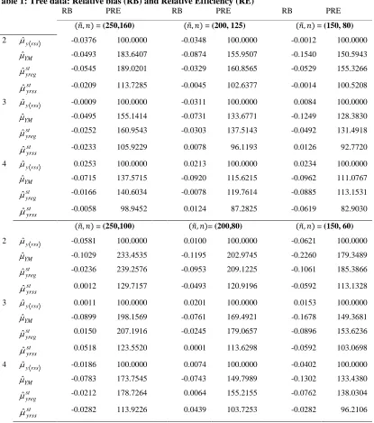
j and PRE t( )j are computed for the five populations with m=2,3, 4 for the live and simulated populations and are given in the Table 1 and Table 2.Table 1: Tree data: Relative bias (RB) and Relative Efficiency (RE)
RB PRE RB PRE RB PRE
(𝑛̃, 𝑛) = (250,160) (𝑛̃, 𝑛) = (200, 125) (𝑛̃, 𝑛) = (150, 80)
2
ˆy rss
-0.0376 100.0000 -0.0348 100.0000 -0.0012 100.0000
ˆYM
-0.0493 183.6407 -0.0874 155.9507 -0.1540 150.5943
ˆst yreg
-0.0545 189.0201 -0.0329 160.8565 -0.0529 155.3266
ˆst yrss
-0.0209 113.7285 -0.0045 102.6377 -0.0014 100.5208
3
ˆy rss
-0.0009 100.0000 -0.0311 100.0000 0.0084 100.0000
ˆYM
-0.0495 155.1414 -0.0731 133.6771 -0.1249 128.3830
ˆst yreg
-0.0252 160.9543 -0.0303 137.5143 -0.0492 131.4918
ˆst yrss
-0.0233 105.9229 0.0078 96.1193 0.0126 92.7720
4
ˆy rss
0.0253 100.0000 0.0213 100.0000 0.0234 100.0000
ˆYM
-0.0715 137.5715 -0.0920 115.6215 -0.0962 111.0767
ˆst yreg
-0.0166 140.6034 -0.0078 119.7614 -0.0885 113.1531
ˆst yrss
-0.0058 98.9452 0.0124 87.2825 -0.0619 82.9030
(𝑛̃, 𝑛) = (250,100) (𝑛̃, 𝑛)= (200,80) (𝑛̃, 𝑛) = (150, 60)
2
ˆy rss
-0.0581 100.0000 0.0100 100.0000 -0.0621 100.0000
ˆYM
-0.1029 233.4535 -0.1195 202.9745 -0.2260 179.3489
ˆst yreg
-0.0236 239.2576 -0.0953 209.1225 -0.1061 185.3866
ˆst yrss
0.0012 129.7157 -0.0493 120.9196 -0.0592 113.1328
3
ˆy rss
0.0011 100.0000 0.0201 100.0000 0.0153 100.0000
ˆYM
-0.0899 198.1569 -0.0761 169.4921 -0.1678 149.3681
ˆst yreg
0.0150 207.1916 -0.0245 179.0657 -0.0896 153.6236
ˆst yrss
0.0518 123.5520 0.0001 113.6298 -0.0592 103.0698
4
ˆy rss
-0.0186 100.0000 0.0074 100.0000 -0.0402 100.0000
ˆYM
-0.0783 173.7545 -0.0743 149.7989 -0.1302 133.4380
ˆst yreg
-0.0212 178.7264 0.0064 155.2155 -0.0762 138.0304
ˆst yrss
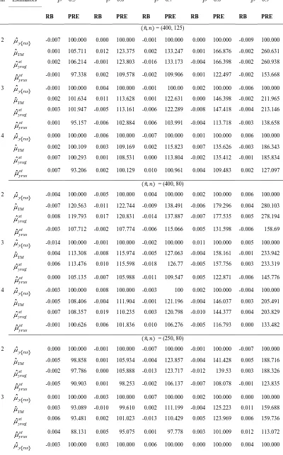
Table 2: Bivariate Normal data: Relative bias (RB) and Relative Efficiency (RE)
m Estimators = 0.5 = 0.6 = 0.7 = 0.8 = 0.9
RB PRE RB PRE RB PRE RB PRE RB PRE
(𝑛̃, 𝑛) = (400, 125)
2 ˆy rss -0.007 100.000 0.000 100.000 -0.001 100.000 0.000 100.000 -0.009 100.000
ˆYM
0.001 105.711 0.012 123.375 0.002 133.247 0.001 166.876 -0.002 260.631
ˆst yreg
0.002 106.214 -0.001 123.803 -0.016 133.173 -0.004 166.398 -0.002 260.938
ˆst yrss
-0.001 97.338 0.002 109.578 -0.002 109.906 0.001 122.497 -0.002 153.668 3 ˆy rss -0.001 100.000 0.004 100.000 -0.001 100.00 0.002 100.000 -0.006 100.000
ˆYM
0.002 101.634 0.011 113.628 0.001 122.631 0.000 146.398 -0.002 211.965
ˆst yreg
0.003 101.947 -0.005 113.161 -0.006 122.289 -0.008 147.418 -0.004 213.146
ˆst yrss
0.001 95.157 -0.006 102.884 0.006 103.991 -0.004 113.718 -0.003 138.658 4 ˆy rss 0.000 100.000 -0.006 100.000 -0.007 100.000 0.001 100.000 0.006 100.000
ˆYM
0.002 100.109 0.003 109.169 0.002 115.823 0.007 135.626 -0.003 186.343
ˆst yreg
0.007 100.293 0.001 108.531 0.000 113.804 -0.002 135.412 -0.001 185.834
ˆst yrss
0.007 93.206 0.002 100.129 0.010 100.961 0.004 109.483 0.002 127.097
(𝑛̃, 𝑛) = (400, 80)
2 ˆy rss -0.004 100.000 -0.005 100.000 0.004 100.000 0.002 100.000 0.006 100.000
ˆYM
-0.007 120.563 -0.011 122.744 -0.009 138.491 -0.006 179.296 0.004 280.103
ˆst yreg
0.008 119.793 0.017 120.831 -0.014 137.887 -0.007 177.535 0.005 278.194
ˆst yrss
-0.003 107.712 -0.002 107.774 -0.006 115.066 0.005 131.598 -0.006 158.69 3 ˆy rss -0.014 100.000 -0.001 100.000 -0.002 100.000 0.011 100.000 0.005 100.000
ˆYM
0.004 113.308 -0.008 115.974 -0.005 127.063 -0.004 158.161 -0.001 233.942
ˆst yreg
0.006 113.476 0.010 115.598 -0.018 126.77 -0.005 157.756 0.003 233.319
ˆst yrss
0.000 105.135 -0.007 105.988 -0.011 109.547 0.005 122.871 -0.006 145.776 4 ˆy rss -0.003 100.000 0.008 100.000 -0.003 100 0.002 100.000 -0.004 100.000
ˆYM
-0.005 108.406 -0.004 111.904 -0.001 121.196 -0.004 146.037 0.003 205.491
ˆst yreg
0.007 108.357 0.019 110.235 0.003 120.798 -0.010 144.377 0.004 203.829
ˆst yrss
-0.001 100.626 0.006 101.836 0.010 106.276 -0.005 116.793 0.000 133.482
(𝑛̃, 𝑛) = (250, 80)
2 ˆy rss 0.000 100.000 -0.001 100.000 -0.007 100.000 -0.001 100.000 -0.007 100.000
ˆYM
-0.005 98.858 0.001 105.934 -0.004 123.857 -0.004 141.428 0.005 188.716
ˆst yreg
-0.002 97.786 0.000 105.888 -0.013 123.717 -0.012 139.53 0.003 188.326
ˆst yrss
-0.005 90.903 0.001 98.253 -0.002 106.137 -0.007 108.078 -0.001 123.835 3 ˆy rss 0.001 100.000 -0.003 100.000 0.007 100.000 0.002 100.000 0.000 100.000
ˆYM
0.003 93.089 -0.010 99.610 0.002 111.199 -0.004 125.223 0.011 159.688
ˆst yreg
0.006 93.481 0.002 101.023 -0.013 110.429 0.005 123.969 0.006 159.736
ˆst yrss
4 ˆ
YM
-0.004 91.438 0.002 95.469 0.012 103.284 0.009 115.114 0.000 139.226 ˆst
yreg
0.007 90.762 -0.001 95.006 -0.002 102.485 -0.003 113.655 0.001 140.013 ˆst
yrss
0.003 86.252 0.002 89.996 0.005 92.301 0.001 95.570 0.002 103.763
3.1. Simulation Results
Relative biases of all the estimators are very low in general. For the tree data it ranges from -0.2260 to 0.0518. The relative biases for the simulated bivariate normal data is much lower than that of the tree data and it varies from -0.014 to 0.023. The estimators and using auxiliary information possess higher relative efficiency than the naïve estimator
in almost all situations. The proposed two-phase stratified regression estimator performs the best, the next place is occupied by two-phase un-stratified regression estimator . The estimator performs the best in all situations for the tree data with a maximum PRE 239.2576. The stratified estimator performs better than naïve estimator in general but in some isolated situations, it possesses lower efficiency (with the minimum PRE = 86.252) than the naïve estimator. For a given combination of (𝑛̃, 𝑛), PREs of all the estimators for both the tree data and simulated data decrease with m. For a given
𝑛̃ and m, PRE of the estimators decreases with n.The relative efficiencies of all the estimators for the simulated data increase with the correlation coefficient . The Yule-estimator performs slightly better than the proposed two-phase estimator in scanty occasions.
4. Conclusion
Stokes (1977) recommended regression estimator for the ranked set sampling when the population mean of the auxiliary variable is known. Yu and Lam (1997) proposed the regression estimator in two-phase sampling when the population mean of the auxiliary variable is unknown. We also propose an alternative two-phase stratified ranked set sampling. On the basis of real and simulated data, it is found that the proposed regression estimator outperforms the other estimators in most situations, especially for the real tree data. We suggest therefore that instead of using phase sampling, one should use two-phase stratified sampling for small strata for improving efficiency of the Yu-Lam estimator. Determination of the asymptotic distribution of the proposed estimators, coverage probabilities of the asymptotic confidence intervals and Bootsrap confidence intervals using Akgul et al. (2018) are subjects of our future research.
Acknowledgement
The authors would like to thank Editor and the referees for their constructive comments and suggestions which improved and enriched the presentation of the paper.
This article was finalized during the R & D leave granted to Prof J. O. Olaomi by the University of South Africa. The views expressed in this paper are those of the authors alone, and they do not necessarily reflect the views of the University of South Africa.
ˆYM
ˆst
yreg
ˆy rss
ˆst
yreg
ˆYM
ˆst
yreg
ˆst yrss
ˆYM
ˆst
yreg
References
1. Akgul, F.G., Acitas,S., and Senoglu, B. (2018). Inferences on stress-strength reliability based on rank set sampling data in case of Lindley distribution. Journal of Statistical Computation and Simulation, 88 (15), 3018-3032.
2. Chen, Z., Bai, Z. Sinha, B.K. (2003). Ranked Set Sampling theory and Applications. Springer, New York.
3. Dell, T.R. and Clutter, J.L. (1972). Ranked-set sampling theory with order statistic background. Biometrics, 28, 545-555.
4. Frey, J., Ozturk, O., and Deshpande, J. (2007). Nonparametric tests for perfect judgment rankings. Journal of the American Statistical Association, 102: 708-717.
5. Kadilar, C., Unyazici, Y. and Cingi, H. (2006). Ratio estimator for the population mean using ranked set sampling. Statistical Papers, 50, 301-309.
6. Mahdizadeh, M. and Zamanzade, E.2018. Stratified pair ranked set sampling. Communications in Statistics-Theory and Methods, 47(24), 5904-5915.
7. McIntyre, G.A. (1952). A method of unbiased selective sampling using ranked sets. Australian Journal of Agricultural Research, 3, 385-390.
8. Platt, W.J., Evans, G.M., and Rathbun, S.L. (1988). The population dynamics of long-lived confier (Pinus plustris). American Naturalist, 131, 491-525.
9. Raghunath Arnab and J. O. Olaomi (2015). Improved estimation from ranked set sampling. Hacettepe Journal of Mathematics and Statistics, 44 (6), 1513 – 1525 10.Stokes, S.L. (1977). Ranked set sampling with concomitant variables,
Communications in Statistics- Theory and Methods, 12, 1207-1211.
11.Stokes, S.L. (1980 a). Inference on correlation coefficient in bivariate normal populations from ranked- set sampling. Journal of the American Statistical Association,75, 989-995.
12.Stokes, S.L. (1980). Estimation of variance using judgment ordered ranked-set samples. Biometrics, 36, 35-42.
13.Takahasi, K. (1970). Practical note on estimation of population means based on samples stratified by means of ordering. Annals of the Institute of Statistical Mathematics, 22, 421-428.
14.Takahasi, K. and Wakimoto, K. (1968). On unbiased estimates of the population mean based on the sample stratified by means of ordering. Annals of the Institute of Statistical Mathematics, 20, 1-31.
15.Yu, P.L.H. and Lam, K. (1997). Regression estimator in ranked set sampling, Biometrics, 53, 1070- 1080.
16.Zamanzade, E., and Al-Omari, A.I. (2016): New ranked set sampling for estimating the
population mean and variance. Hacettepe Journal of Mathematics and Statistics, 45(6), 1881-1905.
17.Zamanzade, E., Arghami, N.R., and Vock, M. 2012. Permutation-based tests of perfect ranking, Statistics and Probability Letters, 82(12), 2213-2220.
18.Zamanzade, E., and Mahdizadeh, M. (2018): Distribution function estimation using concomitant-based ranked set sampling. Hacettepe Journal of Mathematics and Statistics, 47(3), 755-761.
19.Zamanzade, E., and Vock, M. 2018. Some nonparametric tests of perfect