Development of the theoretical and methodological aspects of the singular spectrum analysis and its application for analysis and forecasting of economics data

(1)

Development of the theoretical and

methodological aspects of the singular

spectrum analysis and its application for

analysis and forecasting of economics data

Hossein Hassani

P R t f - Y S G O L

CARP'S*

Cardiff School of Mathematics, Cardiff University

(2)

UMI Number: U585B15

INFORMATION TO ALL USERS

The quality of this reproduction is dependent upon the quality of the copy submitted. In the unlikely event that the author did not send a complete manuscript and there are missing pages, these will be noted. Also, if material had to be removed,

a note will indicate the deletion.

Dissertation Publishing

UMI U585315

Published by ProQuest LLC 2013. Copyright in the Dissertation held by the Author. Microform Edition © ProQuest LLC.

ProQuest LLC

789 East Eisenhower Parkway P.O. Box 1346

(3)

DECLARATION

This work has not previously been accepted in substance for any degree and is not being concurrently subm itted in candidature for any degree. Signed... (candidate) D a te ...

STATEMENT 1

This thesis is being subm itted in partial fulfillment of the requirements for the degree of .Doctor of Philosophy.

Signed (candidate) D a te.

...9*Qet~2c>o9

STATEMENT 2

This thesis is the result of my own investigation, except where otherwise stated. O ther sources are acknowledged by giving explicit reference. A bibliography is .appended.

Signed (candidate) D ate .S .T 7.^?.^...77..?^9?^

STATEMENT 3

I hereby give consent for my thesis, if accepted, to be available for pho tocopying and for inter-library loan, and for the title and summary to be made available to outside organizations. ■ Signed ... (candidate) D a te ... 7

(4)

Abstract

In recent years Singular Spectrum Analysis (SSA), used as a pow erful technique in time series analysis, has been developed and applied to many practical problems. The aim of this research is to develop theoretical and methodological aspects of the SSA technique and to demonstrate th a t SSA can be considered as a powerful method of time series analysis and forecasting, particulary for economic time series.

For practical aspect and empirical results, various economic and financial time series are used. First, the SSA technique is applied as a noise reduction method. The performance of SSA is examined in noise reduction of several im portant financial series. The daily closing prices of several stock market indices are examined to analyse whether noise reduction m atters in measuring dependencies of the financial series. The effect of noise reduction is considered on the linear and nonlinear measures of dependence between two series. The results are compared with those obtained with the linear and nonlinear methods for filtering time series. The results show th a t the performance of SSA is much better than of the competitive methods.

Second, we consider the performance of SSA in forecasting various time series. For consistency with the forecasting results obtained with other current forecasting methods, the performance of the SSA tech nique is examined by applying it to a well-known time series d ata set, namely, monthly accidental deaths in the USA. The results are com pared with those obtained using Box-Jenkins SARIMA models, the ARAR algorithm and the Holt-W inter algorithm. The results show

(5)

th a t th e SSA technique gives a much more accurate forecast than the other methods indicated above.

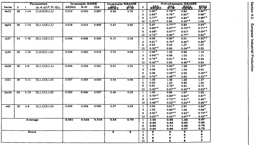
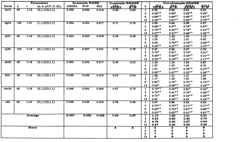
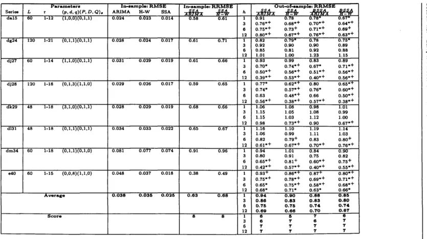
As another example, the performance of the SSA technique is as sessed by applying it to 24 series measuring the monthly seasonally unadjusted industrial production for im portant sectors of the German, French and UK economies. The results confirm th a t at longer horizons, SSA significantly outperforms ARIMA and Holt-W inter methods.

Moreover, the application of SSA to the analysis and forecasting of Iranian national accounts data, which are rather short, are considered to examine capability of SSA in forecasting short time series. The results confirm th a t SSA works very well for short tim e series as well as for long time series.

The univariate and multivariate SSA are also employed in predicting the value and the changes in direction of inflation series for the United States. The consumer price indices, and real-time chain-weighted GDP price index series are used in these prediction exercises. Moreover, our out-of-sample h-step-ahead moving prediction results are compared with the prediction results based on methods such as activity-based NAIRU Philips curve, A R (p), and random walk models w ith the latter as a naive forecasting method. A short-run (quarterly) and long-run (one to six years) time windows are utilized for predictions. The results clearly confirm th a t prediction of inflation rate in the United States during the period of “Great M oderation” is less challenging compared to more volatile inflationary period of 1970-1985 also.

Furthermore, the univariate and multivariate SSA is used for pre dicting the value and the direction of changes in the daily pound/dollar exchange rate. Empirical results show th a t the forecast based on the

(6)

multivariate SSA compares favorably to the forecast of the random walk model both for predicting the value and the direction of changes in the daily pound/dollar exchange rate. The SSA forecasting results are also compared to prediction results based on an error correction model (VEC) in the context of a restricted vector autoregressive model. The results show th a t the VEC results are inferior.

For theoretical development of the technique, two new versions of SSA are introduced; the SSA technique based on the minimum variance estim ator and based on the perturbation theory. The new versions are examined in reconstructing and forecasting time series. The results are compared with the current version of SSA and indicate th a t the new versions improve the quality of reconstruction step as well as forecasting results.

We also consider the concept of casual relationship between two time series based on the SSA technique. We introduce several criteria which characterize this causality. The criteria are based on the forecasting accuracy and predictability of the direction of change. The performance of the proposed test is examined using different real tim e series.

(7)

4 SSA AS A FORECASTING METHOD

39

4.1 American Death series 41

4.1.1 The D ata 41

(8)

Contents ii

4.1.2 Comparison 55

4.2 European Industrial Production 59

4.2.1 The d ata 60

4.2.2 Forecasting Results 62

4.3 Iranian National Account Time Series 74 4.3.1 Analysis of Iranian National Account 74 4.3.2 Analysis of quarterly d ata sets 77

4.3.3 Yearly d ata sets 82

4.3.4 Iranian Inflation rate series 83

4.3.5 Forecasting Iranian Macroeconomics series using

MSSA 85

4.4 Exchange Rate Series 88

4.4.1 The D ata 91

4.4.2 Trend Analysis 92

4.4.3 Results 93

4.4.4 Further Comparisons 98

4.4.5 MSSA results for the Efficient Market Hypothesis 101

4.5 Inflation Rate Series 104

4.5.1 Methods used in the previous studies 108

4.5.2 The d ata 110

4.5.3 Forecasting Inflation rate based on the CPI-all

and CPI-core series 110

4.5.4 Comparison with the other methods 114 4.5.5 Inflation rate based on the GNP and GDP price

index: 1970s to mid-1980s and 1985-2007 119

4.5.6 Discussions 119

(9)

Contents 111

5 SSA BASED ON THE MINIMUM VARIANCE ESTI

MATOR

125

5.1 Introduction 125

5.2 LS and MV Estim ators 127

5.2.1 LS Estim ate of S 128

5.2.2 MV Estim ate of S 129

5.2.3 Weight m atrix W 132

5.3 Separability 132

5.4 Empirical results and comparison 134

5.4.1 Simulated series 134

5.4.2 Real series 136

5.5 Conclusion 138

6 SSA BASED ON THE PERTURBATION THEORY 140

6.1 Introduction 140

6.2 Perturbation Theory 142

6.2.1 Related theorems 142

6.2.2 Subspace method and perturbation theory 143 6.3 SSA based on the Perturbation Theory 152

6.4 Empirical results 154

6.4.1 Simulated d ata 154

6.4.2 Chaotic time series 161

6.4.3 Real d ata 162

6.5 Conclusion 165

7 A COMPREHENSIVE CAUSALITY TEST BASED ON

THE SINGULAR SPECTRUM ANALYSIS

167

(10)

Contents iv

7.2 Causality Criteria 170

7.2.1 Forecasting accuracy based criterion 170 7.2.2 Direction of change based criterion 174 7.3 Comparison with Granger causality test 178

7.3.1 Linear Granger causality test 178

7.3.2 Nonlinear Granger causality test 181 7.3.3 More about the dissimilarity between Granger

causality and the SSA-based techniques 182 7.4 Index of Industrial Production Series 184

7.5 Conclusion 187

8 SUMMARY AN D CONCLUSION

189

A MEASURES OF ACCURACY AND STATISTICAL SIG

NIFICANCE OF THE PREDICTIONS

195

A .l Root mean square of errors (RMSE) 196

A.2 Diebold-Marino significance test 196

A.3 Mean Relative Absolute Error (MRAE) 197

A.4 Direction of change criterion 198

B FILTERING METHODS

199

B.0.1 Autoregressive Moving Average: ARMA 199 B.0.2 Generalized Autoregressive Conditional Heteroskedas-

ticity: GARCH 200

C LINEAR AND NONLINEAR M EASURES OF DEPEN

DENCE

202

C .l Linear correlation coefficient and autocorrelation 202

(11)

Contents V

C.3 Detrended fluctuation analysis 206

C.4 Detrended Moving Average Method 208

D APPLICATION OF SSA FOR THE FABRICATED METAL

SERIES IN GERM ANY

210

E INDUSTRIAL PRODUCTION

SERIES

216

F SEPARABILITY

217

F.0.1 Weak and strong separability 217

(12)

Acknowledgements

I would like to thank my supervisor Professor A. Zhigljavsky, for his invaluable support and guidance throughout this PhD. The creativity and enthusiasm of him for Singular Spectrum Analysis has inspired me to work on this topic.

I am indebted to Dr. V. N etrutkin and Dr. N. Golyandina from St. Pe tersburg University, who have contributed significantly to the provision of m aterials required for this research.

I would like to special thanks Central Bank of the Islamic Republic of Iran for the financial support they have provided throughout this research.

I would also like to thank my external examiner, Prof. C. Ioannidis, and my internal examiner, Dr V. Moskvina, for taking the time to read my thesis and for their useful suggestions th a t led to the improvement of this thesis.

My appreciation and gratefulness to the friendly staff of the Cardiff School of M athematics for their help and kind at various times during my research.

(13)

Acknowledgements Vll

I dedicate this thesis to my wife

M A N S I

who did more than her fair share in life and love while I worked on this thesis. Mansi is my source of strength and w ithout her patient love and her support this work would never have started much less finished.

(14)

Publications

1. Hassani, H. (2007). Singular Spectrum Analysis: Methodology and Comparison. Journal of Data Science, 5(2), pp. 239-257. 2. Hassani, H; Heravi, H; and Zhigljavsky, A. (2009). Forecasting

European Industrial Production with Singular Spectrum Analy sis, International journal of forecasting, 25(1), pp. 103-118. 3. Hassani, H; and Zhigljavsky, A. (2009). Singular Spectrum Anal

ysis: Methodology and Application to Economics D ata, Journal o f Systems Science and Complexity (JSSC), 22(3), pp. 372-394. 4. Hassani, H. (2010). Singular Spectrum Analysis Based on the

Minimum Variance Estim ator, Nonlinear Analysis: Real World Applications, Forthcoming.

5. Hassani, H; Soofi, A; and Zhigljavsky, A. (2010). Predicting Daily Exchange Rate with Singular Spectrum Analysis, Nonlinear Anal ysis: Real World Applications, Forthcoming.

6. Hassani, H; Zokaei, M; von Rosen, D; Amiri, S; and Ghodsi, M. (2009). Does noise reduction m atter for curve fitting in growth curve models?, Computer Methods and Programs in Biomedicine,

96(3), pp. 173-181.

(15)

Publications ix

7. Ghodsi, M; Hassani, H; Sanei, S; and Hicks, Y. (2009). The Use of Noise Information for Detection of Temporomandibular Disorder, Journal of Biomedical Signal Processing and Control, 4(2), pp. 79-85.

8. Hassani, H; Thomakos, D. (2010). A Review on Singular Spec trum Analysis for Economic and Financial Time Series, Statistics and Its Interface, Forthcoming.

9. Hassani, H; Zhigljavsky, A; Patterson, K; and Soofi, A. (2010). A Comprehensive Causality Test Based on the Singular Spectrum Analysis, Causality in Science, Oxford University press, Forth coming.

10. Patterson, K; Hassani, H; Heravi, S; and Zhigljavsky, A. (2010). Forecasting the Final Vintage of the Index of Industrial Produc tion, Journal of Applied Statistics, Forthcoming.

11. Ghodsi, M; Hassani, H; and Sanei, S. (2010). Extracting Fetal Heart Signal From Noisy M aternal ECG by Singular Spectrum Analysis, Statistics and Its Interface, Forthcoming.

12. Hassani, H., Zhigljavsky, A; and Xu, Z. (Subm itted). Singular Spectrum Analysis Based on the Perturbation Theory.

13. Hassani, H; Soofi, A; and Zhigljavsky, A. (Submitted). Predicting Inflation Dynamics with Singular Spectrum Analysis.

14. Sanei, S.; Ghodsi, M; and Hassani, H. (Submitted). A constrained Singular Spectrum Analysis Approach to Murmur Detection from Heart Sounds.

(16)

List of Acronyms

S V D Singular Value Decomposition SSA Singular Spectrum Analysis L R F Linear Recurrent Formula

C D F Cumulative Distribution Function

R W Random Walk

A C F Autocorrelation Function D FA Detrended Fluctuation Analysis D M A Detrended Moving Average

A R M A Autoregressive Moving Average

A R Autoregressive

V A R Vector Autoregressive

G A R C H Generalized Autoregressive Conditional Heteroskedas-ticity

R M S E Root Mean Square Error

(17)

List of Acronyms xi

G D P Gross Domestic Product G N P Gross National Product E M H Efficient Market Hypothesis

(18)

List of Symbols

H

The absolute value of a a.b The dot product of a and b A T The transpose of m atrix A

X T The transpose of vector X

11* 1 1

The Euclidean norm of vector X

I I A I I

f The Frobenius norm of m atrix A

IIA I U

The Euclidean norm of m atrix A ( ,) The inner product

n The last L — 1 components of the vector

y 7

_{The first}_L_{— 1 components of the vector}

£ r

Linear Space

n

Hankelization procedure

V Linear operator

(19)

List of Figures

2.1 An illustration of MSSA. 23

3.1 The daily closing prices of several stock indexes returns: DAX 30,CAC 40, FTSE 100, IBEX 35, S&P 500, PSI 20

and ASE. 38

4.1 Death series: monthly accidental deaths in the USA

(1973-1978). 41

4.2 Principal components related to the first 12 eigentriples. 43

4.3 Logarithms of the 24 eigenvalues. 45

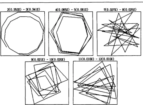
4.4 Scatterplots of the 6 pairs of sines/cosines. 46 4.5 Scatterplots of the paired harmonic eigenvectors. 47 4.6 Periodograms of the paired eigentriples (2-3, 4-5, 7-8,

9-10, 11-12). 48

4.7 M atrix of ^-correlations for the 24 reconstructed com

ponents. 49

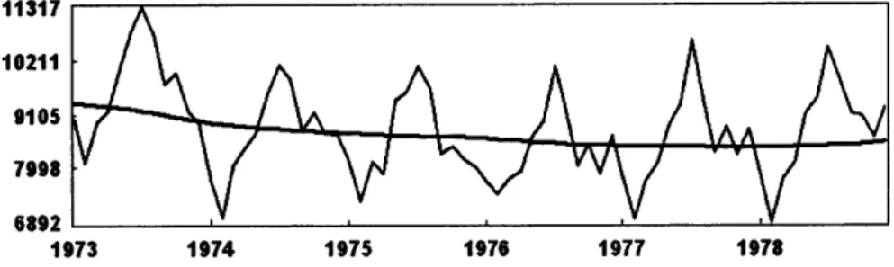
4.8 Trend extraction (first eigentriple). 51 4.9 Trend extraction (first and sixth eigentriples). 51 4.10 Oscillation extraction (eigentriples 2-12). 52 xiii

(20)

LIST OF FIGURES xiv

4.11 Oscillation extraction (eigentriples 2-5,7-12). 4.12 Residual series (eigentriples 13-24).

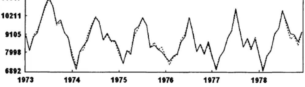
4.13 Reconstructed series (eigentriples 1-12).

4.14 Original series (solid line), reconstructed series (dotted line) and the 6 forecasted d a ta points of 1979.

4.15 The cumulative distribution functions of the absolute values of the out-of-sample errors (for all eight series and 3 countries) obtained by SSA (thick line), ARIMA (thin line) and Holt-W inter (dashed line)

4.16 Series 1-16.

4.17 Series 1-16 in the logarithmic scale. 4.18 Series 17-32.

4.19 Series 17-32 in the logarithmic scale.

4.20 CPI series (left) and inflation rate series based on the CPI series (right) Mar. 1990 - Sep. 2007.

4.21 Iranian GDP deflator (left side) and Iranian G D P /Iranian GDP deflator (right side).

4.22 The exchange rate series UK (thin line) and EU (thick line) exchange rate series over the period 2000 to 2006. 4.23 Trends of UK (thin line) and EU (thick line) rescaled

exchange rate series which are obtained from the first eigentriple.

4.24 Empirical cumulative distribution functions of the ab solute errors for MSSA (thick line) and random walk

(dashed line). 52 53 54 55 68 76 77 78 79 84 86 92 93 98

(21)

LIST OF FIGURES X V

4.25 Empirical cumulative distribution functions of the ab solute errors for MSSA (thick line) and random walk (dashed line) for 1-step ahead (left side) and 3-step ahead forecast (right side) over the period JAN 1997 to Nov 2008.114

5.1 w-correlation between extracted signal and noise series for different window length based on the LS (dashed line)

and MV estimate (thick line). 135

5.2 The performance of SSAm v and SSA^s in reconstruction

(left) and forecasting (right) noisy sin series. 135 5.3 The RRMSE of SSAa/v/SSA^s in reconstruction (left)

and forecasting (right) noisy sin series. 136

6.1 The value of RRMSE in reconstructing of noisy series 5012 (top), 501 (middle) and 51 (bottom) for different

window length. 156

6.2 The value of RMSE in reconstructing of noisy sin for different window length using SSAp t (dashed line) and

SSAL5 (thick line). 157

6.3 The values of RRMES for different noise levels for the

series 5012. 158

series 501. 159

(22)

LIST OF FIGURES xvi

6.6 The value of RRMSE in reconstructing of noisy series for different N; S012 (thick line), SOI (dashed line) and

SI (thin line). 160

6.7 Left: A realization of the series 5012 corrupted with a heteroscedasticity noise. Right: The values of RRMES for different heteroscedasticity noise levels. 161 6.8 The values of RRMES in reconstructing Henon map. 161

D .l Fabricated metal series in Germany 211

D.2 Logarithms of the 120 eigenvalues. 212

D.3 M atrix of w-correlations for the 120 reconstructed com

ponents. 213

D.4 The first 18 principal components plotted as tim e series 214 D.5 Scatterplots (with lines connecting consecutive points)

corresponding to the paired harmonic principal compo

nents. 214

D.6 Reconstructed trend (top), harmonic (middle) and noise

(23)

List of Tables

3.1 The value of ^-correlation for different values of L and r. 30 3.2 The values of the ACF at lag 1, A, c u d f a, and c x d m a of

the Henon map for different noise levels. 30 3.3 Descriptive statistics of several stock indices returns se

ries before and after filtering. 33

3.4 The values of the ACF at lag-1 and A of several stock indices returns series before and after filtering. 33 3.5 The values of p and A of several stock market indices series. 36

4.1 Forecast data, MAE and MRAE for six forecasted d ata

by several methods. 58

4.2 Descriptive statistics of the series. 62

4.3 Descriptive statistics of Out-of-sample and In-sample er rors, UK. * indicates significance for DM test at 10% or less, + indicates significance for encompassing test at

10% or less. 69

(24)

LIST OF TABLES xviii

4.4 Descriptive statistics of Out-of-sample and In-sample er rors, Germany. * indicates significance for DM test at 10% or less, + indicates significance for encompassing test at 10% or less.

4.5 Descriptive statistics of Out-of-sample and In-sample er rors, France. * indicates significance for DM test at 10% or less, + indicates significance for encompassing test at 10% or less.

4.6 Descriptive statistics of out-of-sample errors.

4.7 Out-of-sample percentage of forecasts of correct sign. * indicates significance a t 5% and ** indicates significance at 1%.

4.8 Relative Absolute Error and Mean Relative Absolute Er ror for Series 1 - 1 6 before and after taking th e logarithm 4.9 The RAE and MRAE for Series 1 7 - 3 2 before and after

taking the logarithm.

4.10 RMSE of the SSA forecast results with respect to the RW method, Diebold-Marino significance test results and di rection of change test for inflation rate based on the CPI series.

4.11 MSSA against SSA.

4.12 The MSSA results for different combination.

4.13 Summary of the results for forecasting of UK exchange rate series with SSA and RW. *** indicates the signifi cant results on the 1% level.

70 71 72 73 81 82 85 86 87 96

(25)

LIST OF TABLES xix

4.14 Summary of the results for forecasting of UK exchange rate series with MSSA, VAR and RW. Symbols *, **, and *** indicate the significant results on the 10%, 5%

and 1% levels, respectively. 97

4.15 Augmented Dickey-Fuller test statistics 99 4.16 The results of Cointegration Test. ** denotes rejection

of the hypothesis at the 1% level. 100

4.17 The pairwise Granger Causality Tests. 100 4.18 Summary of the results for forecasting of UK exchange

rate series with MSSA/RW, VAR/RW and MSSA/VAR. Symbols *, **, and *** indicate the significant results on the 10%, 5% and 1% levels, respectively. 101 4.19 RMSE of MSSA forecast results with respect to th e RW

method, Diebold-Mariano significance test results and direction of change test for inflation rate based on the CPI-all and CPI-core series. ** and * imply significance at 1% and 10% confidence levels, respectively. 113 4.20 RMSE of MSSA forecast with other models for 3-month

ahead forecast for 3-month moving averages of inflation rate based on the CPI-all and CPI-core series. AO= Atkeson and Ohanian; AR=Autoregressive; DFM88 =Dy- namic factor model based on 88 variable; DFM158=Dynamic

factor model based on 158 variables. 116

4.21 Direction of change results of 3-month ahead forecasts of the moving average series. * and ** indicate the 10% and 1% levels of significance, respectively. 118

(26)

LIST OF TABLES X X

4.22 The results of DC test and the ratio of root mean squared error (RMSE) of SSA /random walk for the quarterly and annual real-time GNP and GDP chain-weighted price indexes. * and ** indicate the 10% and 1% levels of

significance, respectively. 119

5.1 RRMSE of the post-sample forecasts. 137

5.2 w-correlation and normality test. 138

6.1 Descriptive statistics of several stock indices returns se

ries before and after filtering. 163

6.2 The values of the ACF at lag-1 and A of several stock indices returns series before and after filtering. 163 6.3 The value RRMSE of the post-sample forecasts. 165

7.1 An arrangement of Z x and Zx \y in forecasting n future

points of the series X . 177

7.2 The value of F p ’p - *^ and in forecasting of ith

vintage of the index of industrial production series. 188

(27)

Chapter 1

INTRODUCTION

Econometric methods have been widely used to forecast the evolution of quarterly and yearly national account d ata sets. For example, accurate prediction of inflation rate has been a subject of great research interest for economists. Accurate prediction of inflation plays an im portant role in macroeconomic policy analysis and decision making. However, many of the structural or time series forecasting models have failed to predict accurately economic time series.

On the other hand, many factors could affect the national economies and hence the national account d ata which are a t best inaccurate rep resentation of the macroeconomic variables because of measurement noise. The exogenous factors th a t cause instability in macroeconomics include technological changes, government policy changes, changes in the preferences of the consumers, and other events. These shocks cause structural changes in these time series making them nonstationary. De velopment of a methodology which is robust under these changes, is of paramount importance in accurate prediction of macroeconomic time series.

There are several reasons why classical model does not have a good performance for modelling and forecasting economic and financial se ries. First, an economic model th a t has been established to have validity

(28)

2 in explaining a relationship under one set of assumptions is useless if the assumptions are not valid. Model assumptions include not only those th a t can be expressed as predicates on model parameters but others with more qualitative or asym ptotic form (for more information see [1]).

Moreover, many structural econometric and time series models de vised for forecasting macroeconomic time series are based on restrictive assumptions of normality and linearity of the observed data. The meth ods th a t do not depend on these assumptions could be very useful for modelling and forecasting economics data. On the other hand classical methods of forecasting such as ARIMA type models are based on the assumption such as stationarity of the series and norm ality of residuals (see, for example, [2], [3] and references therein) .

Furthermore, it is well known th at noise can seriously limit accu racy of time series prediction. Currently there are not many effective forecasting techniques available when there is significant noise in the time series data.

In general, there are two main approaches for forecasting noisy time series. According to the first one, we ignore the presence of noise and fit a forecasting model directly from noisy d ata hoping to extract the underlying deterministic dynamics. According to the second approach, which is often more effective than the first one, we start with filtering the noisy time series in order to reduce the noise level and then forecast the new d ata points (see, for example, [4,5] and references therein). There are several linear and nonlinear noise reduction methods such as ARMA model, local projective, singular value decomposition (SVD) and simple nonlinear filtering. It is currently accepted th a t SVD-based

(29)

3 methods are very effective for the noise reduction in deterministic time series and correspondingly for forecasting [5].

Additionally, some of the previous research have considered eco nomic and financial time series as deterministic, linear dynamical sys tems. In this case, the linear models can be used for modelling and forecasting. However, it has been shown th a t most of the financial time series are nonlinear (see, for example, [4-7]); in these cases, we should use nonlinear methods. Having a method th a t works well for both linear and nonlinear, stationary and non stationary time series is ideal for modelling and forecasting. The Singular Spectrum Analysis (SSA) meets all conditions stated above. The SSA technique is a non- parametric technique of time series analysis incorporating the elements of classical time series analysis, multivariate statistics, multivariate ge ometry, dynamical systems and signal processing [8]. Note also th at SSA naturally incorporates the filtering of the series and the SVD.

The appearance of SSA is usually associated with the publication of papers by Broomhead and King [9] while the ideas of SSA were simultaneously developed in Russia (St. Petersburg, Moscow) and in several groups in the UK and USA [8,11]. A thorough description of the theoretical and practical foundations of the SSA technique (with many examples) can be found in [8,10]. An elementary introduction to the subject can be found in [11]. Below we describe several applications of SSA and provide a brief discussion on the methodology used.

The basic SSA method consists of two complementary stages: de composition and reconstruction; both stages include two separate steps. At the first stage we decompose the series and at the second stage we reconstruct the original series and use the reconstructed series for fore

(30)

4 casting new d ata points. The main concept in studying the properties of SSA is ‘separability’, which characterizes how well different compo nents can be separated from each other. The absence of approximate separability is often observed in series with complex structure. For these series and series with special structure, there are different ways of modifying SSA leading to different versions such as SSA with single and double centering, Toeplitz SSA, and sequential SSA [8].

On the other hand, asymptotic separation plays a very important role in the theory of SSA. It has been observed th a t in many practical applications the asymptotic features (which hold as the length of the series T tends to infinity) are met for relatively small values of T; it is not uncommon to successfully apply SSA to series with T equal to 20-30. Another im portant feature of SSA is th a t it can be used for analyzing relatively short series. I has been shown th a t SSA works very well for short time series as well as for long time series in forecasting macro-economics d ata [12].

It is worth noting th a t although some probabilistic and statistical concepts are employed in the SSA-based methods, we do not have to make any statistical assumptions such as stationarity of the series or normality of the residuals. Therefore, SSA is a very useful tool which can be used for solving the following problems:

finding trends of different resolution; smoothing;

extraction of seasonality components;

simultaneous extraction of cycles with small and large periods; extraction of periodicities with varying amplitudes;

(31)

5 finding structure in short tim e series.

Solving all these problems corresponds to the so-called basic capa bilities of SSA. In addition, the method has several essential extensions. First, the multivariate version of the method permits the simultaneous expansion of several time series; see, for example [10]. Second, the SSA ideas lead to several forecasting procedures for time series; see [8,10]. Also, the same ideas are used in [8] and [13] for change-point detection in time series. For comparison with classical methods, ARJMA, ARAR algorithm and Holt-Winter, see [14]- [16]. For autom atic methods of identification within the SSA framework see [17] and for recent work in ‘Caterpillar’-SSA software as well as new developments see [18].

Let us mention some other areas related to SSA. A variety of tech niques of time series analysis and signal processing have been suggested th a t use SVD of certain matrices; for surveys see, for example, [19,20]. Most of these techniques are based on the assumption th a t the original series is random and stationary; they include some techniques th a t are famous in signal processing, such as Karhunen-Loeve decomposition (for signal processing references see, for example [21]). Some statis tical aspects of the SVD-based methodology for stationary series are considered, for example, in [22] and [23,24].

The analysis of periodograms is an im portant p art of the process of identifying the components in the SSA decomposition. A comparison of the observed spectrum of some common time series (these can be found, for example, in [25] and [26], Chapter 11) can help in understanding the nature of the residuals and in the formulation of the proper statistical hypothesis concerning the noise.

(32)

6 The idea of using dynamical systems theory for analyzing financial time series can be justified using the argument th a t the traditional statistical methods have only very limited success in real world financial applications; this is due to the fact th a t the financial time series have very complicated dynamical behaviour, see e.g. [4].

Another area which SSA is related to, is nonlinear (deterministic) time series analysis. It is a fashionable area of rapidly growing popular ity; see, for example, recent books [27-30]. In the area of nonlinear time series analysis SSA was considered as a technique th a t could compete with more standard methods. There is a number of studies th a t consid ered SSA as a filtering method in (see, for example, [31] and references therein). The superiority of the SSA technique over traditional digital filtering methods used in biomedical data was shown, with several ex amples in the literature [32]. In another study, the noise information extracted using the SSA technique, has been used as a biomedical di agnostic test [33]. The SSA technique also used as a filtering method for longitudinal measurements. It has been shown th a t noise reduction is im portant for curve fitting in growth curve models, and th a t SSA can be employed as a powerful tool for noise reduction for longitudinal measurements [34].

Here we use the SSA technique for analysis, filtering, and forecasting financial and economic time series. The univariate and multivariate version of the SSA technique is used in this predictions which include both the magnitude and direction of changes.

The structure of this thesis is as follows. A brief introduction of the SSA method is represented in C hapter 2. In Chapter 3, we consider the SSA technique as a noise reduction method. The performance of

(33)

7 SSA as a forecasting method is considered in Chapter 4. Two new versions of SSA, SSA based on th e minimum variance estimator and SSA based on the perturbation theory, are introduced in Chapters 5 and 6. A new casuality test based on the SSA technique is introduced in Chapter 7. Finally, Chapter 8 presents a summary of the study and some concluding remarks.

(34)

Chapter 2

SINGULAR SPECTRUM

ANALYSIS

The main purpose of SSA is to decompose the original series into a sum of series, so th a t each component in this sum can be identified as either a trend, periodic or quasi-periodic component (perhaps, amplitude- modulated), or noise. This is followed by a reconstruction of the original series. The Basic SSA technique is performed in two stages, both of which include two separate steps as follows:

f Step 1 : Embedding Stage 1 : Decomposition

Step 2 : Singular Value Decomposition (SVD)

Stage 2 : Reconstruction Step 1 : Grouping

Step 2 : Diagonal Averaging

A short description of the SSA technique is given as follows (for more information see [8]).

(35)

Section 2.1. Decomposition 9

2.1 Decomposition

1st step: Embedding

Embedding can be regarded as a mapping th a t transfers a one-dimensional time series Yp = {yi, . . . , yp) into the multidimensional series X\ , . . . , with vectors X i = (?/»,..., 2/*+l-i)t £ R l , where K = T — L +1. Vec tors X i are called L-lagged vectors (or, simply, lagged vectors). The single parameter of the embedding is the window length L, an integer such th a t 2 < L < T. The result of this step is the trajectory matrix

2/1 2/2 2/2 2/3 2/3 2/4 \ Ul 2/l+i UL+2 2Ik 2 /f c + i 2 /T

)

Note th a t the trajectory m atrix X is a Hankel m atrix, which means th at all the elements along the diagonal i+ j = const are equal. Embedding is a standard procedure in time series analysis. W ith the embedding performed, future analysis depends on the aim of the investigation. For specialists in dynamical systems, a common technique is to obtain the empirical distribution of all pairwise distances between the lagged vec tors X i and X j and then calculate the so-called correlation dimension of the series. Note th a t in this approach, L must be relatively small and K must be very large (formally, K —* oo ). The approximation of a stationary series with the help of the autoregression model can also

(36)

be expressed in terms of embedding: if we deal with the model

Vi+L-1 = a L -lV i+ L -2 H--- !■ a lVi + £»+L-1> * > 1

then we search for vector A = ( a i , . . . , a ^ -i, — 1)T such th at the scalar products (Xi, A) are described in terms of certain noise series.

2nd step: Singular Value Decomposition (SVD)

The second step, the SVD step, makes the singular value decomposition of the trajectory matrix X and represents it as a sum of rank-one bi- orthogonal elementary matrices. Denote by Ai , . . . , Al the eigenvalues of X X T in decreasing order of magnitude (Ai > . . . A^ > 0) and by

U \ , . . . , U L the orthonormal system of the eigenvectors of the matrix

X X T corresponding to these eigenvalues. Set

d = max(z, such th a t A* > 0) = rank X.

If we denote Vi = X TU i/y /\i, then the SVD of the trajectory matrix can be written as:

X = X x + ---1- X d, (2.1.1)

where X* = V X iU iVjT. The matrices X , have rank 1 (thus they are elementary matrices); C/» (in SSA literature they are called ‘factor em pirical orthogonal functions’ or simply EOFs) and Vi (often called ‘prin cipal components’) are the left and right eigenvectors of the trajectory matrix. The collection (\/Ai, Ui,Vi) is called the i-th eigentriple of the matrix X , y/Xi (i = 1, . . . , d) are the singular values of the m atrix X and the set {>/At} is called the spectrum of the m atrix X. If all eigenvalues

(37)

have multiplicity one, then the expansion (2.1.1) is uniquely defined. SVD (2.1.1) is optimal in the sense th at among all the matrices X(r) of rank r < d, the m atrix Yli=i ^ provides the best approxi mation to the trajectory m atrix X , so th a t || X — X(r) || is mini mum. Here the norm of a m atrix

Y

is defined as y /

(Y, Y),

where the scalar product of two matrices

Y

= (y ij)fj=1 and Z = (zij)ij=i is

(Y,

Z> = £ £ = 1yijZij. Note th a t || X ||2 = £ t i Af and || X t ||2 = As for i = 1 Thus, we can consider the ratio Aj/J^jLi ^i 85 the characteristic of the contribution of the m atrix X* to expansion (2.1.1). Consequently, 5^i=i ^*/ 5Z?=i the sum the first r ratios, is the characteristic of the optimal approximation of the trajectory matrix by the matrices of rank r.

Another optimal feature of the SVD is related to the properties of the directions determined by the eigenvectors C/i,. . . , £/<*. Specifically, the first eigenvector U\ determines the direction such th a t the variation of the projections of the lagged vectors into this direction is maximum. Every subsequent eigenvector determines the direction th a t is orthog onal to all previous directions, and the variation of the projection of the lagged vectors onto this direction is also maximum. Therefore, it is natural to call the direction of the z-th eigenvector Ui the i-th principal direction. Note th a t the elementary matrices X* are built up from the projections of the lagged vectors onto the z-th particular directions. This view on the SVD of the trajectory m atrix composed of Zr-lagged vectors and an appeal to association with the principal component anal ysis lead to the following terminology. We shall call the vector Ui the z-th eigenvector, the vector Vi will be called the i-th factor vector and the vector Z* = y/\iVi the i-th principal component.

(38)

Section 2.2. Reconstruction 12

2.2 Reconstruction

1st Step: Grouping

The grouping step corresponds to splitting the elementary matrices into several groups and summing the matrices within each group. Let 7 = {zi, . . . , ip} be a group of indices i\ , . . . , ip. Then the matrix X j corresponding to the group 7 is defined as X j = X»x H 1- X*p. The spilt of the set of indices J = { 1 , . . . , d} into disjoint subsets I \ ,. . . , 7m corresponds to the representation

X = X /j H b X /m. (2.2.1)

The procedure of choosing the sets 7i, . . . , 7m is called the eigentriple grouping. For a given group 7 the contribution of the component X / in the expansion (2.2.1) is measured by the share of the corresponding eigenvalues: \ / Y li=i -V If the m atrix X / is a Hankel matrix, then there exist series and such th a t Yp = Y ^ + Y ^ and the trajectory matrices of these series are X / and X j\/ , respectively. If the matrices X / and Xj\j are approximately Hankel matrices then the trajectory matrices of the series Y .P and Y ,P are close to X / and X j\/. In this case we shall say th a t the series are approximately sep arable, see [8] for many more details. Therefore, the purpose of the grouping step (that is, the procedure of arranging the indices 1, . . . , d into groups) is to find several groups 7i, . . . , 7m such th a t the matrices X / j , . . . , X / m satisfy (2.2.1) and are close to certain Hankel matrices. The grouping step is based on the analysis of the eigenvectors Ui and

Vi, and eigenvalues A* in the SVD expansion. The principles and meth ods of identifying the SVD components for their inclusion into different

(39)

Section 2.2. Reconstruction 13

groups are described in [8], Sect. 1.6. Since each m atrix component of the SVD is completely determined by the corresponding eigentriple, we shall talk about the grouping of the eigentriples rather than the grouping of the elementary matrices X*.

2nd Step: Diagonal averaging

The purpose of diagonal averaging is to transform a m atrix to the form of a Hankel m atrix which can be subsequently converted to a time series. If Zij stands for an element of a m atrix Z, then the A;-th term of the resulting series is obtained by averaging over all i , j such th a t i + j = k + 1. This procedure is called diagonal averaging, or Hankelization of the m atrix Z. The result of the Hankelization of a matrix Z is the Hankel m atrix TiZ. Note th a t the Hankelization is an optimal procedure in the sense th a t the m atrix TiZ is the nearest to Z (with respect to the matrix norm) among all Hankel matrices of the corresponding size (see [8], Sect. 6.2). In its turn, the Hankel m atrix

TiZ uniquely defines the series by relating the value in the diagonals to the values in the series.

If z ^ stands for an element of a matrix Z, then the A;-th term of the resulting time series is obtained by averaging z ^ over all i, j such th at i + j = k + 2. This procedure is called diagonal averaging, or Hankelization of the m atrix Z. The result of the Hankelization of a matrix Z is the Hankel m atrix TiZ, which is the trajectory matrix corresponding to the time series obtained as a result of the diagonal averaging.

(40)

Section 2.2. Reconstruction 14 L < K in the following way: for i + j = s and N = L + K — 1 the element of the m atrix TiZ is

1 f \ Zi a—l 2 < S < L - 1, * _ 1 w 1 L - y zifS—i L < s < K + 1, 1=1 1 L y zt s—i K + 2 < s < K + L. - s + 1 . ’ K + L — 5 + _ _—/C

Note th a t the Hankelization is an optimal procedure in the sense th a t the m atrix TiZ is the nearest to Z (with respect to the Frobenius norm) among all Hankel matrices of the corresponding size. Note th at the Frobenius norm is equal to the square root of the m atrix trace of X X T. The Hankel m atrix TiZ uniquely defines th e time series by relating the values in the diagonals to the values in th e series.

By applying the Hankelization procedure to all m atrix components of (2.2.1), we obtain another expansion:

X = X /l + . . . + X /m (2.2.2)

where X /x = TiX. This is equivalent to the decomposition of the initial series Yt — ( y i,. . . , Vt) into a sum of m series:

m

y, = Y , y i k) <2-2-3)

fc=i

where = (y[k\ . . . , corresponds to the m atrix X /fc. A sensible grouping leads to the decomposition (2.1.1) where the resultant ma trices X /fc are almost Hankel ones. This corresponds to approximate separability and implies th at pairwise scalar products of different

(41)

ma-Section 2.3. Reconstruction Algorithm 15

trices X /fc in (2.2.2) are small. The procedure of computing the time series (that is, building up the group Ik plus diagonal averaging of the matrix X /fc) will be called reconstruction of a series by the eigentriples with indices in /*. In relation to the grouping method, it is worthwhile to note th a t if L is large enough, the eigenvectors in a sense imitate the behavior of the corresponding time series components. In particular, the trend of the series corresponds to slowly varying eigen vectors. The harmonic component produces a pair of left (and right) harmonic eigenvectors with the same frequency, etc.

2.3 Reconstruction Algorithm

To formalize the SSA reconstruction step, let us have a time series

Yt = (2/1, • • • , 2/r)- Fix L (L < T /2), the window length, and let

K = T - L + 1.

S tep 1. (Computing the trajectory matrix): transfers a one-dimensional time series Yt = (2/1, . . . , 2/t) into the multi-dimensional series X i ,. . . , Xk

with vectors X i = (yi}. . . ,yi+L_ i)' e R L, where K = T — L +1. Vec tors X{ are called L-lagged vectors (or, simply, lagged vectors). The single parameter of the embedding is the window length L, an integer such th a t 2 < L < T. The result of this step is the trajectory matrix

x = [*„...,*•*] = (*„)j£r

S te p 2. ( Constructing a matrix fo r applying SVD): compute the matrix X X T .

S te p 3. (SVD of the matrix X XT): compute the eigenvalues and eigen-vectors of the m atrix X X T and represent it in the form X X T = P A P T. Here A = diag(Ai , . . . , Al) is the diagonal matrix of

(42)

Section 2.4. Forecasting Algorithm 16

eigenvalues of X X T ordered so th a t Ai > A2 > . . . > A^ > 0 and

P = (Pi, P2, . . . , P l) is the corresponding orthogonal matrix of eigen vectors of X X T.

S te p 4. (Selection of eigen-vectors): select a group of / (1 < / <

L) eigen-vectors Pix, P»2, . . . , Pit.

The grouping step corresponds to splitting the elementary matrices

X{ into several groups and summing the matrices within each group. Let I = {f 1, . . . , ii} be a group of indices fy,. . . , ii. Then the matrix X / corresponding to the group I is defined as X / = X ^ H X ir

S te p 5. (Reconstruction of the one-dimensional series): com pute the m atrix X = ||x<j|| = Ylk=i 33 an approximation to X. Transition to the one-dimensional series can now be achieved by averaging over the diagonals of the m atrix X.

2.4 Forecasting Algorithm

Forecasting by SSA can be applied to the time series th a t approximately satisfy linear recurrent formulae (LRF):

d

yi+d = akyi+d- k, 1 < i < T - d (2.4.1)

k = 1

of some dimension d with the coefficients An important property of the SSA decomposition is that, if the original time series

Yt satisfies a LRF, then for any T and L there are a t most d nonzero singular values in the SVD of the trajectory m atrix X; therefore, even if the window length L and K = T - L + 1 are larger than d, we only need at most d matrices X* to reconstruct the series.

(43)

speaking, states that: If the number of terms r in the SVD of the tra jectory matrix X is smaller th an the window length L, then the series satisfies some LRF of some dimension d < r. Let us formally describe the forecasting algorithm under consideration (for more information see [8]):

Algorithm input:

(a) Time series YT = (yl f . . . , yT).

(b) Window length L, 1 < L < T.

(c) Linear Space £ r C R L of dimension r < L. It is assumed that

cl £ £ r , where eL = ( 0 , 0 , . . . , 1) E R L. (d) Number M of points to forecast.

Notations and comments-.

(a) X = [X i, . . . , Xk\ is the trajectory m atrix of the time series Yt.

(b) P i , . . . , Pr is an orthonormal basis in £ r .

(c) X = [Xj : . . . : X K] = T h e vector X { is the orthogonal projection of X i onto the space £ r .

(d) X = H X = [X\ : : Xk\ is the result of the Hankellization of the m atrix X.

(e) For any vector Y E R L we denote by Y h E R L_1 the vector consisting of the last L — 1 components of the vector V, while Y 7 E R L" J is the vector of the first L — 1 components of the vector Y .

(f) We set u2 = 7Tj + . . . + 7if, where 7t* is the last component of the vector Pi (i = 1 , . . . , r).

(g) Suppose th a t eL i £ r (This implies th a t £ r is not a vertical space). Then v2 < 1. It can be proved th a t the last component t/l of

(44)

any vector Y = (3/1, , Vl)T £ £ r is a linear combination of the first components (yu . . . , 2/z,-i) :

Vl - a iyL -i + •. • +

Vector A = ( a i , . . . , aL-i) can be expressed as

i = l

and does not depend on the choice of a basis P\ , . . . , Pr in the lin ear space £ r . In the above notations, define the tim e series Yt+m =

(2/1, , Vt+m) by the formula

V i = <

Vi for i = 1 , . . . , T

(2.4.2)

The numbers yr+i, • • • , 2/t+m from the M terms of the SSA recurrent forecast. Let us define the linear operator V ^ : £ r t—► R L by the formula

■p(r)y _

Y1 L X a t y k , V G £ r Set for i = 1, . . . , K (2.4.3)

the m atrix Z = [Zi , . . . , Zk+m] is the trajectory matrix of the series

(45)

Section 2.5. Bootstrapping 19

2.5 Bootstrapping

Assume th a t we have a time series Yt = {yt}J=1 = where

y£1} is the signal and represents the noise. Let us consider a method of constructing average series for the signal Vt\m at time T+M.

In the unrealistic situation, when we know both the signal Y ^ and the true model of the noise Y j? \ the Monte Carlo simulation can be applied to check the statistical properties of the forecast values y^+M relative to the actual term .

Indeed, assuming th a t the rules for the eigentriple selection are fixed, we can simulate N independent copies Y }?■ (i = 1 , . . . , i V) of the process Y ^ and apply the forecasting procedure to N independent time series YT)i = + Y^2- . Then the forecasting result will form a sample 2/T+M,t> which should be compared against Vt+m- this way the Monte Carlo average series for the forecast can be built up.

Since in practice we do not know the signal Y j} \ we can not apply this procedure. Under a suitable choice of the window length L and the corresponding eigentriples, we have the representation Yt = Y ^ + Y p 2\

where YjP (the reconstructed series) approximates Y^ , and YjP is the residual series. Suppose now th a t we have a (stochastic) model for the residual Y jP (for instance, we can postulate some model for Y ^ and, since Y ^ « Y^l\ we apply the same model for Y ^ with the estimated parameters). Then, simulating N independent copies Yj?) of the series

Yj?^, we obtain N series Yt j = Y ^ + Y ^ } and produce M forecasting

results Vr+Mi in the same manner as in the Monte Carlo simulation variant.

From the sample Vt+m *(1 < i < N ) of the forecasts we can compute the average bootstrap forecast. This average bootstrap can then be

(46)

Section 2.6. Confidence intervals for th e forecasts 20

compared with the value y r\.M obtained by Basic SSA forecast. Large discrepancy between these two forecasts would typically indicate th at the original SSA forecast is not reliable. Furthermore, using the sample of the bootstrap forecast results we can estimate the distribution of the forecasts and compute, for example, confidence intervals for the true values. To do th at, we need a stochastic model for Yp2^; a standard assumption would be the assumption th a t is a Gaussian white noise. This assumption can be easily verified using the classical tests for randomness and normality.

2.6 Confidence intervals for the forecasts

Confidence intervals for the forecasts can be calculated by two meth ods: the empirical method and the bootstrap method (which is also an empirical method). They are calculated using the residuals of the reconstruction.

According to the main SSA forecasting assumption, the component

Y±l) of the series Yt has to satisfy an LR F of a relatively small dimen sion, and the residual series YjP = Yp — Y ^ has to be approximately separable from Y p \ In particular, y / 1^ is assumed to be a finite sub series of an infinite series y ^ \ which is a recurrent continuation of Y p \

These assumptions are often hold in practice with high accuracy. There are two problems related to the construction of the confidence intervals for the forecast. The first problem is to construct a confidence interval for the original series Yp = {yt} at some future point in time. The second problem is construction of confidence intervals for the sig nal Yp1] = {s/f1^} at some future point in time. These two problems can be solved in different ways. The second requires additional

(47)

infor-Section 2.6. Confidence intervals for the forecasts 21

mation about the model governing the series to perform a bootstrap simulation of the series Yt- Bootstrap confidence intervals

are built for the continuation of the signal Y ^ (for more information see [8]).

Let us consider a method of constructing intervals for the signal

Y $ lM at the moment T+M . In the unrealistic situation, when we know both the signal Y ^ and the true model of the noise Yp2\ a Monte Carlo simulation can be applied to check the statistical properties of the forecast value i/t+m relative to the actual term Vt+m

-Indeed, assuming th a t the rules for the eigentriple selection are fixed, we can simulate N independent copies Y ^ } {i = 1,2, ••• ,JV) of the process YjP and apply the forecasting procedure to N indepen dent time series Yt,{ = YjP + Y ^ . Then the forecasting result will form a sample Vt+m.v which should be compared against Vt+m- this way the Monte Carlo average series for the forecast can be built up. Since in practice we do not know the signal Y j} \ we can not apply this procedure. Let us describe the bootstrap variant of the simulation for constructing the confidence intervals for the forecast.

Under a suitable choice of the window length L and the correspond ing eigentriples, we have the representation Yt = Y ^ + Y p 2\ where Y ^

(the reconstructed series) approximates Y ^ , and Y jP is the residual series. Suppose now th a t we have a (stochastic) model for the residual Yp2) (for instance, we can postulate some model for Y ^ and, since

Yj.1^ ~ Yj.1^, we apply the same model for Y ^ with the estimated pa rameters). Then, simulating N independent copies Y ^ of the series

Y ^ p, we obtain N series Yr,i = Y ^ + Y ^ } and produce M forecasting results *n the same manner as in the Monte Carlo simulation

(48)

Section 2.7. Multivariate singular spectrum analysis (MSSA) 22

variant.

More precisely, any time series Yt,% produces its own recon structed series and its own forecasting linear recurrent formula LRFi

for the same window length L and the same sets of eigentriples. Start ing at the last L - 1 terms of the series , we perform M steps of forecasting with the help of its LRFi, to obtain

From the sample i (1 < i < N ) we can calculate its (empirical) lower and upper quintiles for a fixed level 7 and obtain the correspond ing confidence interval for the forecast. This interval (called bootstrap confidence interval) can be compared with the forecast value ob tained from the initial forecasting procedure. We can also build average bootstrap series. This average can then be compared with the value

Vt+m obtained by Basic SSA forecast. Large discrepancy between these

two forecast would typically indicate th a t the original SSA forecast is not reliable.

The simplest model for is the Gaussian white noise model. The corresponding hypothesis can be checked with the help of the standard test for randomness and normality.

2.7 Multivariate singular spectrum analysis (MSSA)

The use of multivariate singular spectrum analysis (MSSA) for multi variate time series was proposed theoretically in the context of nonlinear dynamics in [9]. There are numerous examples of successful application of the multivariate SSA (see, for example, [1] and [10]). Multivariate (or multichannel) SSA is an extension of the standard SSA to the case of multivariate time series. We give a short description of MSSA method as follows.

(49)

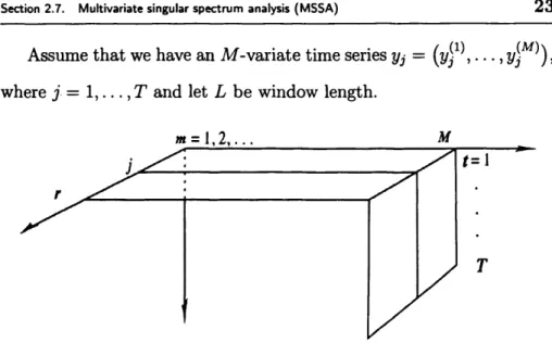
Assume th a t we have an M -variate time series yj = ( y f \ • • ., VjM^) > where j = 1 , . . . , T and let L be window length.

F ig u re 2.1. An illustration of MSSA.

Similar to univariate version, we can define the trajectory matri ces (i = 1 , . . . , M ) of the one-dimensional time series { y ^ } (i =

1 , . . . , M) . The trajectory matrix X can then be defined as

X =

<

x<» ^

X (M>

J

(2.7.1)

Fig. 2.1 shows an illustration of MSSA. The structure of matrix C = X X T is as follows: f C n .

Clm

• C \m ^

c

=

cml

.

•

Cmm

CmM

^

C m i • C M m • Cm m J (2.7.2)

where, C u = X (/)(X (,7))T (/, J = 1, . . . , M) is an estimate of the co- variance between two trajectories X ^ and X ^ corresponding to the

(50)

series Y 1 and Y J. The other stages of multivariate SSA procedure are identical to the basic SSA as described above with an obvious modifi cation th at the diagonal averaging should be applied to each of the M

(51)

Chapter 3

SSA AS A NOISE

REDUCTION METHOD

In this chapter, the daily closing prices of several stock market indices are examined to analyse whether noise reduction m atters in measuring dependencies of the financial series. We consider the effect of noise reduction on the degree of the linear and nonlinear measure of depen dencies between to time series. We also use SSA as a powerful method for filtering financial series. The results are compared with those ob tained by ARMA and GARCH models as linear and nonlinear methods for filtering the series. We also examine the findings on an artificial data set namely the Henon map.

3.1 Introduction

During the last few years the analysis of financial time series has re ceived increasing attention. Many researchers have discovered evidence for the possibility th a t the financial markets may be nonlinear dynam ical systems, with im portant implications in the Efficient Market Hy pothesis. Several researchers, by using different statistical tests, have mentioned evidence of non-independently and identically distributed

(52)

Section 3.1. Introduction 26

behaviour of the financial time series, and also the existence of the nonlinear dependence among these series [35]- [43].

Several measures have been used to calculate the degree of indepen dency or dependency. The most known measure to calculate depen dency between two random variables is the coefficient of linear correla tion, but its application requires a pure linear relationship, or at least a linear transformed relationship. This statistics may not be helpful in determining serial dependence if there is some kind of nonlinearity in the d ata [44,45].

Urbach [46] defends a strong relationship between entropy, depen dence and predictability. This relation has been studied by many au thors [45]- [48]. It has been shown th at a measure based on the mutual information, which captures linear and nonlinear dependencies, without requiring the specification of any kind of model of dependence, is better than the linear correlation coefficient to measure serial correlation of several stock market indices [44]- [48].

Recently, two new methods have been developed to measure long- range correlations in non-stationary fluctuating series; the detrended fluctuation analysis [49,50] and the detrended moving average method [51,52]. These methods detect persistency by assuming the self-similarity of the series.

It is well known th a t the existence of a significant noise level reduces the efficiency of the methods to analyze financial time series. Consider a time series yt = st + et (t = 1, . . . , T) which behaves as stochastic dynamic systems with both a deterministic element, st, and a stochastic part et. We consider the second part as noise. Here we investigate the efficiency of noise reduction on the measures of dependencies (linear

(53)

Section 3.1. Introduction 27

and nonlinear).

We mainly follows two different approaches to calculate the mea sures of dependence. According to the first one, we calculate the mea sures of dependencies directly from the noisy time series. Therefore, we ignore the existence of the noise in the first approach. According to the second approach we start with filtering the noisy time series in order to reduce the noise level and then calculate the measures. It is clear th a t the results by the second approach are more effective than the first one if we select a proper method for filtering the series.

There are several nonlinear methods for filtering noisy series such as local projective, Digital Butterworth filters, splines, filters based on spectral analysis, singular value decomposition (SVD) and simple nonlinear filtering. It has been shown th a t the SVD-based methods are more effective than the other ones for the reduction of noise in financial time series [53]. Here, we use the SSA technique as a tool for filtering financial time series. Recent research shows th a t SSA can be used as an alternative to traditional filtering methods [31]. For example, Alonsoa [32] showed superiority of the SSA te