2014
A local structure graph model for network analysis
Emily Taylor Casleton
Iowa State University
Follow this and additional works at:
http://lib.dr.iastate.edu/etd
Part of the
Statistics and Probability Commons
This Dissertation is brought to you for free and open access by the Graduate College at Digital Repository @ Iowa State University. It has been accepted for inclusion in Graduate Theses and Dissertations by an authorized administrator of Digital Repository @ Iowa State University. For more
information, please [email protected].
Recommended Citation
by
Emily Taylor Casleton
A dissertation submitted to the graduate faculty in partial fulfillment of the requirements for the degree of
DOCTOR OF PHILOSOPHY
Major: Statistics
Program of Study Committee: Mark S. Kaiser, Co-Major Professor Daniel J. Nordman, Co-Major Professor
Petrut¸a C. Caragea Arka P. Ghosh Max D. Morris Alyson G. Wilson
Iowa State University Ames, Iowa
2014
DEDICATION
I would like to dedicate this thesis to my husband, Dave, without whose support, patience, encouragement, and whiteboard discussions I would not have been able to complete this work.
TABLE OF CONTENTS
LIST OF TABLES . . . vi
LIST OF FIGURES . . . viii
ACKNOWLEDGEMENTS . . . xii ABSTRACT . . . xiii CHAPTER 1. INTRODUCTION . . . 1 1.1 Background . . . 1 1.2 Overview . . . 3 1.2.1 Literature Review . . . 3
1.2.2 The Local Structure Graph Model (LSGM) . . . 3
1.2.3 LSGM with Higher-Order Dependence . . . 4
1.2.4 Importance of Transitivity . . . 4
CHAPTER 2. LITERATURE REVIEW . . . 6
2.1 Introduction . . . 6
2.2 Graph Analysis: Algorithmic construction . . . 8
2.2.1 Random Graph Models . . . 12
2.2.2 Small World Models . . . 14
2.2.3 Preferential Attachment . . . 16
2.3 Graph Analysis: Probabilistic modeling . . . 19
2.3.1 Exponential Random Graph Models . . . 20
CHAPTER 3. A LOCAL STRUCTURE MODEL FOR NETWORK
ANAL-YSIS . . . 51
3.1 Introduction . . . 51
3.2 Exponential Random Graph Model (ERGM) . . . 53
3.3 Local Structure Graph Model (LSGM) . . . 56
3.3.1 Specification . . . 57
3.3.2 Model Parameters . . . 61
3.3.3 Additional Features . . . 65
3.4 Application . . . 68
3.4.1 The Network . . . 68
3.4.2 The Fit of the LSGM . . . 70
3.4.3 Model Assessment . . . 71
3.5 Conclusions . . . 74
CHAPTER 4. LOCAL STRUCTURE GRAPH MODELS WITH HIGHER-ORDER DEPENDENCE . . . 76
4.1 Introduction . . . 77
4.2 Parameterization for MRF Models . . . 79
4.2.1 Original Parameterization . . . 80
4.2.2 Centered Parameterization . . . 81
4.3 Parameterization for Random Graph Models . . . 82
4.4 Higher-Order Dependence . . . 85
4.4.1 Centering of Third Summation in LSGM . . . 87
4.5 Example . . . 90
4.5.1 Inclusion of Attributes . . . 90
4.5.2 Inclusion of Higher-Order Terms . . . 94
4.6 Conclusions . . . 100
4.7 Appendix . . . 102
4.7.1 Proof of Proposition 4.3.1 . . . 102
CHAPTER 5. DATA STRUCTURES REPRESENTED BY A RANDOM
GRAPH MODEL: WHEN IS TRANSITIVITY NEEDED? . . . 105
5.1 Introduction . . . 105
5.2 Example Networks . . . 106
5.3 Models . . . 109
5.4 Exploratory Data Analysis of Networks . . . 113
5.5 Analysis . . . 117
5.6 Discussion . . . 126
CHAPTER 6. GENERAL CONCLUSIONS . . . 128
6.1 General Discussion . . . 128
6.2 Recommendation for Future Research . . . 129
LIST OF TABLES
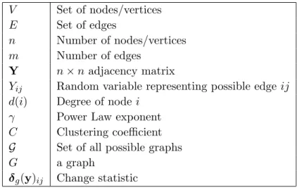
Table 2.1 Comparison of the strengths and weaknesses of the two categories of probabilistic modeling: exponential random graph models (ERGMs) and latent variable models (LVMs). . . 20 Table 2.2 Table of notation used within the literature review of Chapter 2. . . . 50
Table 3.1 Point estimates and 90% percentile parametric bootstrap interval es-timates for the LSGM and independence model fits to the Arkansas tornado network. . . 71
Table 4.1 Parameter estimates and 90% percentile parametric bootstrap confi-dence intervals for the LSGM fit to the Buell-Small succession network. 93 Table 4.2 Conditional expectations for both Japanese honeysuckle and red sorrel
edges based on the number of positive neighbors. Values in red are less than the corresponding marginal expectations. . . 94 Table 4.3 Parameter estimates and 90% percentile parametric bootstrap
confi-dence intervals for the football networks. . . 98 Table 4.4 Characterization of the cliques of size three for the 2000 and 2013
foot-ball networks as the proportion of cliques of size three for which none, one, or both other edges assume the same value as the focal edge and p-values for the distributions in Figure 4.6. . . 100
Table 5.1 Structural comparison of the Faux Mesa High and football networks . 115 Table 5.2 Number of potential 2-stars which can form either zero or one triangle. 116
Table 5.3 Comparison of the realized structures of the Faux Mesa High and foot-ball networks. . . 117 Table 5.4 Parameter estimates and 90% percentile parametric bootstrap
confi-dence intervals for three models fit to the Faux Mesa High network. . . 118 Table 5.5 Parameter estimates and 90% percentile parametric bootstrap
confi-dence intervals for three models fit to the football network. . . 119 Table 5.6 Marginal and conditional expectations for edges with the potential
LIST OF FIGURES
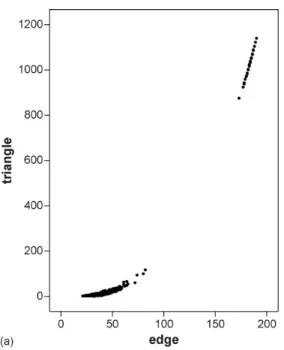
Figure 2.1 Demonstration of the Small-World model of Watts and Strogatz (1998). The graphs increase in randomness from right to left. . . 15 Figure 2.2 Configuration of edges which leads to partial conditional dependence. . 25 Figure 2.3 Scatterplot of number of edges against the number of triangles from a
simulation study conducted by Robins et al. (2007) for an ERGM with density parameter fixed at -1.5 and triangle parameter ranging from 0 to 1. . . 38 Figure 2.4 An example 5-triangle . . . 40
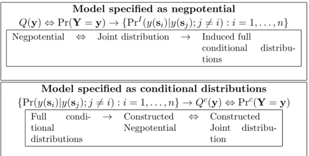
Figure 3.1 Two example networks and dependence structures with resulting depen-dence graphs. The nodes of the dependepen-dence graph corresponds to the edges of the original graph. An edge in the dependence graph indicates conditional dependence between the two random variables. . . 58 Figure 3.2 Relationship between the negpotential, joint distribution, and full
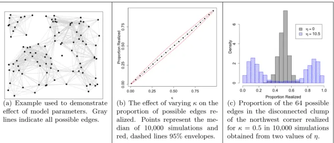
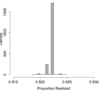
con-ditional distributions when either the model is specified as the negpot-netial or full conditionals. . . 60 Figure 3.3 Example network and a demonstration of the effect of model parameters. 61 Figure 3.4 Proportion of realized edges in 10,000 simulations when κ = 0.5 and
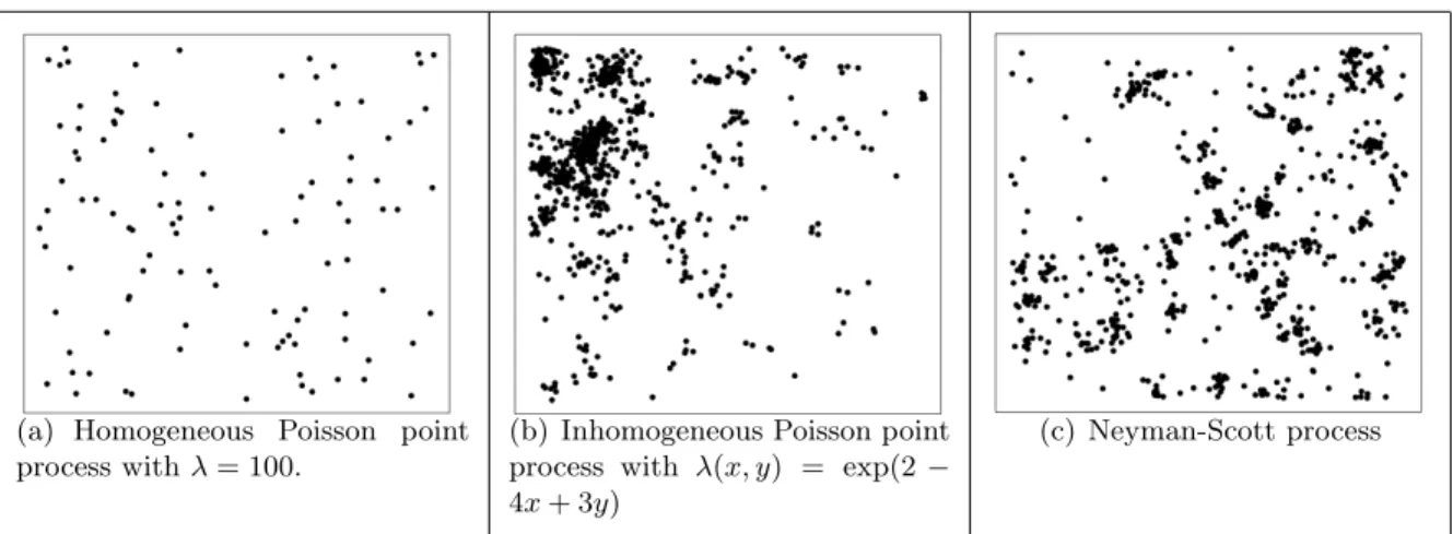
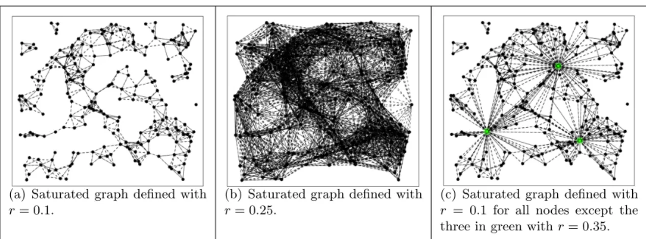
η= 35. The proportion realized does not correspond to the large-scale parameter, κ = 0.5. This is an example of an area of the parameter space where the model is degenerate. . . 64 Figure 3.5 Examples of random node placements through different point processes. 66 Figure 3.6 Examples of saturated graph on same set of nodes for various radius sizes. 67
Figure 3.7 Nodes of the Arkansas tornado network defined by tornadoes that orig-inated in Arkansas during April, 2011. Color and numbers correspond to the event in which the tornado occurred. . . 69 Figure 3.8 Neighborhood sizes when a saturated graph ofr= 80 kilometers is used
in the analysis of the Arkansas tornado network. . . 70 Figure 3.9 Proportions of neighbors assuming the same value as the random
vari-able,q(si) for the Arkansas tornado network. . . 73
Figure 3.10 Number of positive neighbors against conditional expectation for a ran-dom variable with 20 neighbors. The red, dashed, vertical line represents the marginal expectation of ˆκ= 0.27. . . 75
Figure 4.1 Simulation study to show the effect of the centering of the third-order term on a 20×20 lattice. Points represent the average proportion of realized edges (as an approximation of marginal expectationE[Y(si)])
with 90% confidence intervals. . . 89 Figure 4.2 Explanation of neighborhood definition used in the Buell-Small
succes-sion study example. Each sets of five plots represent the same spatial locations. The black, solid line represents the focal edge, and the gray, dashed lines are its neighbors. . . 91 Figure 4.3 Proportion of neighbors of the same species which are realized in 1000
simulations from the model fit in Table 4.1. . . 95 Figure 4.4 Nodes of the college football network and their classification based on
conference (with a slight geographic adjustment to the University of Hawai’i). . . 97 Figure 4.5 Marginal and conditional expectations for the fitted models to the 2000
Figure 4.6 Model assessment of the fits to the 2000 and 2013 football datasets. Boxplots represent proportion of cliques of size three with the corre-sponding number of edges having the same value as the edge of interest from 1000 simulated networks. Red points represent the proportions from the realized networks. . . 101
Figure 5.1 Visualization of the networks of the Faux Mesa High and football network.107 Figure 5.2 Subgraphs which correspond to cliques of size 3 given an incidence
def-inition of dependence: a 3-star (left) and triangle (right). . . 113 Figure 5.3 Neighborhood sizes resulting from the neighborhood definitions of the
Faux Mesa High and football networks. . . 114 Figure 5.4 Histograms of the number of cliques of size three to which the unique
2-stars belong for both the Faux Mesa High and football networks. . . 116 Figure 5.5 Normal quantile-quantile plots of the different proportions from the
sim-ulations from the three models fits to both network. The first row rep-resents simulations from the fit to the Faux Mesa High network and the second row to the football network. The dashed horizontal line repre-sents the proportion from the realized network. A vertical line at the theoretical quantile of zero has been drawn for reference. . . 120 Figure 5.6 Possible configurations used to compute the conditional expectations for
Female–Female and Male–Male (left) and Female–Male (right) in Table 5.6. The focal edge for which the conditional expectation is computed is the dashed line in both. . . 122 Figure 5.7 Conditional expectations for the three models based on number of
pos-itive neighbors. Approximate marginal expectation for each model is plotted as a gray, dashed horizontal line. . . 124
Figure 5.8 Normal quantile-quantile plots which demonstrate the ability of the three models to recreate the 2-stars and triples of dependent edges mod-eled in each of the Faux Mesa High and football networks. Vertical, dashed lines correspond to the actual . . . 125 Figure 5.9 Scatterplot of the estimates ofη2 against η3 for the 839 simulations of
ACKNOWLEDGEMENTS
I would like to take this opportunity to express my thanks to those who helped me with various aspects of conducting research and the writing of this thesis. First and foremost, my advisers, Dr. Dan Nordman and Dr. Mark Kaiser, for their guidance, patience, and support. I have learned a lot from working with them, and I feel I am a much better statistician now than when we began this process with that first trip to Albuquerque. I would like to thank my committee members for their time and patience: Dr. Max Morris, Dr. Petrut¸a Caragea, and Dr. Arka Ghosh. Also, I would like to thank Cindy Phillips and the team at Sandia National Laboratory for motivating the research in network analysis and for funding this work through a Laboratory Directed Research and Development grant.
I would like to thank others who have helped me succeed at Iowa State. To my cohort of fellow graduate students, I would not have made it through the first few years without you. I have heard that the people you attend graduate school with become your colleagues, and I hope I have the opportunity to work with each of you in the future. And to my pod-mates, Adam and Dan, your advice, elaborate motivation, and company on coffee runs has helped me tremendously. Most importantly, I would like to thank the Department of Statistics for encouraging a collegial environment and their continued support and development of graduate students.
Last, but not least, I would like to thank Dr. Alyson Wilson who played a large part in my decision to attend ISU and is the reason I got involved in the project that lead to this thesis. I also greatly appreciate her mentoring and advice throughout my graduate career.
ABSTRACT
The statistical analysis of networks is a popular research topic with ever widening appli-cations. In this work, we introduce a new class of models for network analysis, called local structure graph models (LSGMs). The approach specifies a network model through local fea-tures and allows for an interpretable and controllable local dependence structure. In particular, LSGMs are formulated by a set of full conditional distributions for each network edge, e.g., the probability of edge presence/absence, which depend functionally on neighborhoods or subcol-lections of other network edges. Hence, LSGMs correspond to a type of Markov Random Field (MRF) model applied to graph edges. The modeling features and interpretation of LSGMs are demonstrated through several numerical studies and illustrated through a network data example involving tornado occurrences. LSGMs are also shown to provide an alternate specifi-cation of another popular class of models for random graphs, belonging to exponential random graph models (ERGMs), which specify a model through a joint distribution on the entire col-lection of graph edges. An ERGM induces conditional distributions and neighborhoods, rather than explicitly defining them as in the LSGM approach. As one consequence of its conditional specification, LSGMs have the advantage of allowing direct control and separate interpretation of parameters influencing large-scale (e.g., marginal means) and small-scale (i.e., dependence) structures in a graph model. This is possible with LSGMs through so-calledcentered parameter-izations of MRF models, which ERGMs are shown to lack. The centered parameterization and conditional specification of LSGMs further provide important advantages in graph modeling when incorporating covariate information from nodes, as illustrated with two further network data examples. However, the centered parameterization was developed for MRFs under an as-sumption of pairwise-only dependence, meaning that dependence is modeled between pairs of dependent edges only. This particular dependence structure may be inappropriate for modeling network data that exhibit transitivity or a prevalence of triangles within the network, which
has been identified as an important feature of various networks. Consequently, the centered parameterization for MRFs is extended to account for triples of dependent edges in LSGMs. This extension then allows for the explicit modeling of transitivity in LSGMs, while retaining the same interpretable separation and control of large- and small-scale effects in a graph model and facilitating the use of covariate information. At the same time, the ability to model tran-sitivity does not imply that this model feature should be commonly used or applied without cautious model diagnostics, which are currently lacking for graph models and for ERGMs in particular. By developing simulation-based model assessments for random graphs, we provide in-depth examinations and analyses of two commonly-used example networks, demonstrating that real network data may not, in fact, support the inclusion of transitivity in a graph model.
CHAPTER 1. INTRODUCTION
1.1 Background
Since the mid-1990’s, there has been a research explosion in the area of network science. There are conferences, (e.g., the International Network for Social Network Analysis annual conference, the Intra-Organizational Networks conference, and the annual international con-ference on Advances in Social Network Analysis and Mining), network analysis centers (e.g., Duke Network Analysis Center, LINKS Center for Social Network Analysis at the University of Kentucky, and the Center for Computational Analysis of Social and Organizational Systems at Carnegie Mellon University), special issues of journals (e.g., volume 21, issue 4 of Journal of Computational and Graphical Statistics (2012), volume 21, issue 3 of Journal of Statistical Software(2008), and the inaugural issue of the journalNetwork Science appeared in 2013), and computational packages (e.g., Stanford Network Analysis Project, thestatnetsuite (Goodreau et al., 2008) andergm(Hunter et al., 2008b) packages in R, SIENA (Snijders et al., 2006), and Statistical modeling of sOCial NETwork (StOCNET)).
However, network analysis predates this recent increase in interest. Visualization of graphs as points and lines, known as a sociogram, was introduced by Moreno in 1934 (Fienberg, 2012). One of the first social networks arose from an experiment conducted by Stanley Milgram in the early 1960s which measured the number of connections between two randomly chosen individuals through chain letters. Although a large majority of chains were never completed, Milgram discovered the median length of completed chains was only 6, inspiring the play and movie Six Degrees of Separation (Goldenberg et al., 2010). Probability models for networks can be traced to the Erd¨os-R´enyi-Gilbert graph in 1959 (Kolaczyk, 2009) and the International Network for Social Network Analysis, an association for social-network researchers, was founded
over three decades ago in 1977 (INSNA, 2013). Although the value of networks has long been known, it is only recently that their potential has been realized due to the combination of recent advances in computational ability, which makes analysis of large networks possible, and the emergence of large, freely-available, and interesting networks, such as the Internet, Facebook, or the Wikipedia.
A network is defined by a set of nodes and the relations between them. Networks model relational data, or data with features that cannot be described by only examining the in-dividual nodes (Handcock, 2003a). Complex patterns of connections and dependencies can be represented by a network and between a potentially large number of nodes. Due to this ability, applications from a wide variety of disciplines have been appropriately modeled as a network. For example, biologists have modeled the structural connectivity of brains with net-works (Sporns et al., 2004; Simpson et al., 2011), zoologists use graph models to represent the social network of animals, such as dolphins (Lusseau, 2003), international relations between countries have been analyzed with networks (Hoff and Ward, 2005; Barigozzi et al., 2010), and epidemiologists use networks to understand the spread of a disease within a population (Groendyke et al., 2012). In addition, networks have represented the effect of disasters on fiber-optic networks (Neumayer and Modiano, 2010), the communications between a cell of a terrorist networks (Schweinberger and Handcock, 2012), the reliability of sampled data on a protein-protein interaction networks (Raftery et al., 2012), and the inter-organizational collab-orations between rescue and relief organizations in response to the September 11, 2001 attack (Schweinberger et al., 2012).
This wide variety of applications from various disciplines demonstrates the flexibility of networks as a modeling tool. However, this diverse array of problems has led to a diverse array of solutions from a diverse array of disciplines. As one review aptly described, “Network science has no home” (Vivar and Banks, 2012). Many of the models or methods developed for the analysis of networks have been for a specific application or observed network, and thus most are very ad hoc and not appropriate for other types of observed networks (Vivar and Banks, 2012). This dissertation will present a newly-constructed class of models for the statistical analysis of observed graphs, local structure graph models (LSGMs), which were not developed
for a specific application, but rather is an application of the binary Markov Random Field (MRF) model to graph edges.
1.2 Overview
1.2.1 Literature Review
Network science is vast with published works appearing in a diverse array of fields. Due to extensive and broad range of existing literature, a comprehensive review is not possible, so the literature review presented in Chapter 2 will focus on the contributions from computer scientist/statistical physics and sociologists/statisticians; two subsets of network science that have contributed a considerable amount. The reasons for choosing these two areas is that motivation for this dissertation was a collaboration with a team of computer scientists at Sanida National Laboratory and it was desired to understand the current work relevant to our collaborators. A majority of statisticians working on network analysis have focused on social networks, and thus the goals of the literature in the area of sociology are similar to those of this dissertation.
1.2.2 The Local Structure Graph Model (LSGM)
The new class of models for network analysis, LSGMs, will be introduced in Chapter 3. There are two distinguishing features of a LSGM. The first is the specification, for each poten-tial edge, of a conditional distribution, i.e., the distribution for the presence/absence of that edge given the outcomes of all other potential edges in the network. An explicit definition of dependent sets of edges, called neighborhoods, is the second characteristic of a LSGM. Markov dependence is assumed so that edges are conditionally dependent only on edges that belong to the same neighborhood. Two additional features of LSGMs, the ability to simply incorporate potential spatial information about nodes, and the definition of a “saturated graph,” are also introduced. These features can help keep the potential sizes of LSGM neighborhoods manage-able which helps avoid a common issue of model degeneracy. This chapter will also show that
a LSGM can be interpreted as an alternate method of specifying another model for random graphs, an exponential random graph model (ERGM).
1.2.3 LSGM with Higher-Order Dependence
A LSGM is based on an application of the binary MRF model to the edges of a network. A MRF model is generally used to analyze geo-referenced data because of its ability to incorporate spatial dependence. This dependence is often modeled between pairs of random variables only, an assumption known as pairwise-only dependence, which is sufficient to spatial applications. However, this assumption creates a limitation in specifying conditional distributions for graph edges in LSGMs where it may be necessary to incorporate dependence between triples of depen-dent edges. Another consideration is the parameterization of conditional distributions which can have an important effect on model parameter interpretation. LSGMs have the advantage of allowing direct control and separate interpretation of parameters influencing large-scale (e.g., marginal means) and small-scale (i.e., dependence) structures in a graph model due to the use of a so-called centered parameterization. However, this parameterization was also developed under the pairwise-only dependence assumption. Thus, Chapter 4 extends the centered param-eterization to allow for higher order dependence and shows that the parameter interpretation advantage is maintained.
1.2.4 Importance of Transitivity
The extension introduced in Chapter 4 allows for a LSGM to explicitly model dependence between triples of dependent edges. For an incidence definition of dependence, the common dependence structure in network analysis where two edges that do not share a node are condi-tionally independent, the two topological features that lead to triples of dependent edges are 3-stars and triangles. Modeling transitivity, the prevalence of triangles within the network, has received a lot of attention due to the perceived prevalence in various networks of interest and intuitive scientific interpretation. For example, in a social network, transitivity is demonstrated through two individuals who are more likely to be friends when they share a common friend. Although the idea of transitivity is intuitive, effects that are modeled need to be supported by
the data structures. In Chapter 5, two networks which are commonly used as examples in the literature are studied in detail. These two particular networks were chosen because they allow for a comparison between too little and too much realized structure. Specifically of interest is if the data supports the inclusion of transitivity, or dependent triples of edges in each situation. Simulation-based model assessments, indicate that real network data may not, in fact, support the inclusion of transitivity in a graph model, indicating a need for cautious model diagnostics.
CHAPTER 2. LITERATURE REVIEW
2.1 Introduction
The literature review presented in this chapter will examine a subset of the research pub-lished in the fields of computer science and statistical physics and sociology and statistics. These two areas have made considerable contributions to the advancement of network science. The chapter will not include an exhaustive list of the random graph models from these areas, as network science is vast and quickly evolving in all disciplines. Although there exists multiple literature reviews of network analysis (e.g., Vivar and Banks, 2012; Fienberg, 2012; Goldenberg et al., 2010; Salter-Townshend et al., 2012; Chakrabarti and Faloutsos, 2006), this review is unique in its classification of the network analysis techniques into algorithmic construction and probabilistic modeling.
Most modern models for random graphs arose from the often misinterpreted Erd¨os-R´enyi graph model. Two specifications of this model were proposed at approximately the same time in 1959. In a series of papers, Erd¨os and R´enyi (Kolaczyk, 2009) specified a random graph model where the number of nodes, n, and the number of edges, m, are fixed, and a uniform distribution is placed on allN possible graphs, where
N = n 2 m .
In the same year, Gilbert (1959) proposed his specification of the same model where the number ofnnodes are fixed and edge formation occurs according to a constant, independent probabil-ity p for each of the n2 pair of nodes. From this specification, the likelihood of a particular graph can be determined and is the binomial distribution. Unjustly, Gilbert’s specification is often referred to as the Erd¨os-R´enyi graph. Some works do acknowledge Gilbert’s contri-bution, referring to this model as the Erd¨os-R´enyi-Gilbert model, and it has also been called
the Bernoulli graph (Handcock, 2003a), Poisson model (Chakrabarti and Faloutsos, 2006), or classical random graph model (Kolaczyk, 2009).
A network model is defined by Kolaczyk (2009) as the collection
{Pθ(G), G∈ G;θ∈Θ} (2.1)
where G is the set of all possible graphs and Pθ is a probability distribution over G with
parameter vector θ. Three common approaches to specifying the model,Pθ(G), are discussed.
The first is to restrict the set of graphs,G, under consideration by specifying a set of features, such as a fixed number of nodes or edges. As in the specification of Erd¨os and R´enyi,Pθis then
specified as a uniform distribution over the resulting set of possible graphs. The next approach to specifying the model in (2.1) is to inducePθ through an algorithmic generating mechanism
that simulates a graph. Random variables are often assigned to components of the generative process and probability distributions specified for the random variables. A limitation of this method from a statistical viewpoint is the often lack of a likelihood function for the entire graph. Although the generative algorithm may inducePθ, in most instances it is prohibitively
difficult to formulate and is rarely attempted. The last approach is to explicitly specify Pθ by
associating subgraph configurations and covariate information with graph topology of interest. This approach is taken by many statisticians in the field of network analysis. As a final note, the three approaches to model specification are not mutually exclusive, nor do they encompass all possibilities. For instance, the Erd¨os-R´enyi-Gilbert model can be interpreted within all three categories, and some generative methods have only partial probability structures, thus, it is not clear how to take a generated graph and perform a probability analysis.
There are various possible categorizations of network analysis approaches. Those discussed here will be categorized as algorithmic construction or probabilistic modeling, where the dis-tinguishing characteristic is the interest in a likelihood function. Methods under the heading of algorithmic construction involve the development of an algorithm-based graph generators that can quickly simulate a network which resembles an observed network of interest as much as possible with respect to features deemed to be important. They utilize the first two approaches
of network model specification and either a likelihood function cannot be identified or there is a lack of interest.
The goal of those methods under probabilistic modeling is “statistical model building” (Kolaczyk, 2009) and are defined by a likelihood. Probabilistic models for random graphs are specified by the third approach discussed above. These approaches allow for the estimation of parameters that provide a logical representation of the data and a method to evaluate and compare the fit of the competing models.
A network, or graph, is defined by a set of n nodes and m edges. Most of the discussion will focus on simple graphs, i.e., graphs with unweighted edges and no self-loops, with edges that can be directed or undirected. Graphs are observed at a single point in time, ignoring recent work on dynamic aspects of networks. LetV represent the set of vertices, or nodes and E the set of edges between pairs of nodes. A graph will be represented asG with edge values collected into Y, an n×n adjacency matrix, with each entry Yij a binary random variable
designating the presence, Yij = 1, or absence, Yij = 0, of an edge between nodes i and j. A
realization of the graph will be represented as y.
2.2 Graph Analysis: Algorithmic construction
The defining feature of the graph analysis techniques discussed in this section is the absence of a likelihood function for the graph, either from a lack of consideration or from an inability to discern its functional form. This work has been published largely in the computer science and statistical physics literature where the focus is on the ability to generate realistic graphs. Researchers in this area have condensed observed networks into common, seemingly important features where the goal of the proposed graph-generation algorithm is to quickly generate a graph with as many of the important features as possible. These algorithms may have parameters to be set and there is often probability involved in the formation and deletion of edges; however, given an observed network, these models do not have an ability to estimate values for the parameters, quantify uncertainty, or account for measurement error.
The motivation for developing algorithmic graph generators is to gain an understanding of the processes that lead to the formation of a network of interest (Leskovec et al., 2010)
because often the network to be analyzed is observed at a single point in time. Intuitively, if the algorithm results in a graph comparable to the network of interest, it is plausible that the observed graph arose as a result of operations similar to those performed by the algorithm. Understanding the graph formation procedure can lead to an ability to detect abnormalities in another observed network, allow one to compress a large network while preserving important features (Chakrabarti and Faloutsos, 2006), or to extrapolate and test out scenarios on graphs which cannot be observed (Leskovec et al., 2010), e.g., the Internet in five years.
Three features are commonly observed in realistic networks (Lancichinetti et al., 2008): a power law degree distribution, a small diameter, and clustering. Generators aim to emulate these three features exactly as they appear in a network of interest, in addition to as many other features as possible. For example, a recently proposed algorithm boasts the ability to simulate graphs which match realistic networks on 11 network characteristics (Goldenberg et al., 2010). Only the three generally agreed upon, important features will be described below.
The degree of a node is the number of edges incident, or connecting to, the node (Salter-Townshend et al., 2012). In an undirected graph, the degree of nodei,d(i), is found by summing over either theith row or column of the adjacency matrix,d(i) =Y+j =Pnj=1Yij. The degree
distribution is the collection of degrees for all nodes in the graph,{d(1), d(2), . . . , d(n)}. Many networks of interest contain a few nodes with a large degree while a majority of the nodes have a small degree. In a social network, this is manifested as a few popular people, e.g., celebrities, with a lot of connections and ordinary people with fewer connections. In a graph of the Internet, there are a few websites to which many other sites link, e.g., Wikipedia, Google, while the vast majority have substantially fewer. This phenomena suggests the degree distribution is heavily right skewed, or, as is more commonly described, follows a power law with probability density function of the form
p(d(x)) =A×d(x)−γ (2.2)
where A >0 is a normalizing constant and γ >1 is the power law exponent. Networks with this property are referred it as scale-free graphs (Ben-Avraham et al., 2003). The value of γ is often used as a metric to determine how well the algorithm is able to replicate the degree
distribution of the observed network (Bar et al., 2007). However, estimation of the exponent is not straightforward nor is its computation consistent. Chakrabarti and Faloutsos (2006) list seven of the more commonly used methods.
The second important feature is a measure of graph connectedness. Distance between two nodes can be defined as the number of edges on the shortest path between them. If no such path exists, the distance is defined to be infinity. A graph is connected if all distances are finite and unconnected otherwise. The diameter of a graph is the maximum distance between all pairs of nodes (Gross and Yellen, 2006). For an unconnected graph, either the maximally connected subgraph or the effective diameter can be considered (Salter-Townshend et al., 2012), where the effective diameter is the minimum number of edges between some percentage of nodes (Chakrabarti and Faloutsos, 2006). The diameter in empirical networks has been found to be quite small, especially compared to the size of the network, resulting in the “small-world” effect. For example, Watts and Strogatz (1998) examined a graph with 225,226 movie actors as nodes with an edge between actors in the same film. Using the maximally connected subgraph, the diameter was found to be 3.65, making Kevin Bacon seem less impressive. In the same work, the US power grid represented as 4,941 nodes is found to have a diameter of only 18.7.
Clustering is the final important feature for graph generators to replicate. This phenomena refers to the large number of triangles in an empirical network and is also referred to as tran-sitivity. In a social network, the interpretation of transitivity is that two individuals are more likely to be friends if they share a common friend. Newman et al. (2002) claim the probability of edge formation between two nodes is several orders of magnitude greater if those nodes have a distance of two between them. The amount of clustering is represented by the clustering coefficient, C, which quantifies the proportion of the connected sets of three nodes, or triples, which are closed and thus form a triangle,
C= 3×Number of triangles
Number of connected triples. (2.3)
Empirical networks have been found to have a larger value of a clustering coefficient than if edges formed independently and at random. The movie actor example (Watts and Strogatz, 1998) has a clustering coefficient of 0.79, so 79% of connected triples are triangles. The authors
contrast this with a single graph of the same number of nodes and edges generated by placing the edges at random which resulted in a clustering coefficient of 0.00027.
Some limitations to the graph generation algorithmic approach to network analysis have been identified in the literature. First, although the algorithms attempt to recreate as many features of the empirical networks as possible, there is no consideration if these features are sufficient or necessary descriptions of network structure (Fienberg, 2012). The important fea-tures are chosen because they appear frequently in observed graphs, although recent analysis suggests some features are not as ubiquitous as previously believed (Goldenberg et al., 2010). In fact, Bar et al. (2007) suggest that the power law degree distribution demonstrated in the Autonomous Systems (AS) network, a crucial component of Internet connectivity, may be a consequence of the manner in which the data were collected. Descriptions used to summarize the algorithms do not explore the full parameter space (Goldenberg et al., 2010), and parame-ters are given as point estimates without any quantification of uncertainty. Thus, it is possible that the summary quantities of the realistic networks are highly inaccurate (Fienberg, 2012).
Statistical methods for estimating the model parameters of observed data are also lacking (Fienberg, 2012). When statistical methods are used, they are often applied incorrectly or in violation of assumptions. As an example, to estimate the power law exponent for a degree distribution, γ in (2.2), the distribution is plotted on a log-log scale and the slope is obtained either through ordinary least squares or visual inspection. This approach is used even in the presence of strong non-linearity (Goldenberg et al., 2010). Further, measurement error or other potential biases in the data are not considered. Bar et al. (2007) suggest that up to 50% of the edges in the AS network are not observed; however, even with this acknowledgement, the authors claim they “cannot model data that are unknown.”
Despite the statistical limitations of graph generating algorithms, they have been given a lot of attention in the statistical physics and computer science literature. In 2010, Kolaczyk (2010) speculated that at least 2/3 of the published work on network analysis focused on descriptive methods and as Goldenberg et al. (2010) stated, “Alternative graph generation mechanisms appear [in the literature] every day.” A few historically important and illustrative examples of
the graph generating algorithms will be presented below. Many of the algorithms not included were formulated as slight variations of those discussed.
2.2.1 Random Graph Models
Random graph models (RGMs) are those for which the set of possible graphs G has been defined and equal probability is place on each graph, G ∈ G (Kolaczyk, 2009). These are formulated according to the first common approach of defining the network model, (2.1). A RGM is completely determined by identifying the set of plausible graphs, G, which can be accomplished in two ways: by explicitly stating the set or by determining the possible graphs that could arise from a graph generating algorithm.
In the context of a RGM, the Erd¨os-R´enyi-Gilbert model is often referred to as the “classical random graph model” or just the random graph. As mentioned previously, the Erd¨os-R´ enyi-Gilbert model can be cast as all three types of graph model formulation for (2.1). In addition, the specifications from Erd¨os and R´enyi and from Gilbert can be used to demonstrate the two ways of defining the set G. Under the specification of Erd¨os and R´enyi, the set G contains graphs with a fixed number of nnodes and m edges. Gilbert’s specification can be considered a graph generation scheme, a phenomena referred to by Goldenberg et al. (2010) as “pseudo-dynamic,” where models that were originally proposed to describe a single, static network can be interpreted as a generative algorithm. For Gilbert’s specification of the Erd¨os-R´enyi-Gilbert model, the process begins with n disconnected nodes. At each iteration of the algorithm, a pair of nodes is considered and an edge is added between them with probability p = m/ n2
, independent of all previous iterations. This continues until all pairs of nodes are considered. The set of nodes remain fixed and once an edge is added, there is no mechanism to remove it. The setG resulting from each specification will be equivalent as n→ ∞.
One reason the Erd¨os-R´enyi-Gilbert model has received so much attention is that many of its properties can be calculated exactly (Newman et al., 2002), specifically the identification of a “phase change” (Fienberg, 2012) or “phase transition” (Chakrabarti and Faloutsos, 2006), which occurs atλ=pn= 1. When λ <1, graphs contain small, disconnected groups of edges. The phase associated with λ > 1 is characterized by one giant component (Fienberg, 2012),
which occurs when a majority of the nodes are highly connected (Kolaczyk, 2009). This phase is more commonly observed in empirical networks, and Newman et al. (2002) add the existence of a giant component to the list of features of a realistic network. A direct result of the giant component is the small-world property. However, Erd¨os-R´enyi-Gilbert graphs with λ >1 fail to reproduce the other two important features (Chakrabarti and Faloutsos, 2006). The degree distribution is Binomial and approaches a Poisson asn→ ∞and therefore, the graphs resulting from the generative method are not scale-free. In addition, because edges form independently, so do triangles, and thus the graphs lack the desired clustering. Often, the Erd¨os-R´enyi-Gilbert model is used as a “straw-man” model for newly-proposed algorithms.
In order to address some of the shortcomings of the classical RGM, one proposed solution is to further restrict G to only graphs that contain an important, omitted feature. Graph generation algorithms of this type are called generalized RGMs. Modifications to the setG are intended to produce graphs with features such as small clusters of highly connected nodes, more realized triangles (Fienberg, 2012), or most commonly, a specified degree distribution (Aiello et al., 2001). For this last type of restrictions, the number of nodes and the degree distribution of the graph are fixed, which only allows for a specific number of vertices. Thus, the set of possible graphs for this type of generalized random graph model is a subset of those allowed under the Erd¨os-R´enyi-Gilbert model, given Erd¨os and R´enyi’s specification.
The method to simulate a graph with a specified number of nodes and a degree distribution is as follows. Begin with a graph of n unconnected nodes. Each node is randomly assigned a degree. Nodes are then joined until none of the nodes have any extra degrees. The stan-dard algorithms developed to perform this last step are the matching algorithm and switching algorithm (Kolaczyk, 2009).
Similar to a classical RGM, mathematical properties can be solved in the limit of large n for a generalized RGM that fixes the degree distribution. Specifically, if the degree distribution is defined as a power law, (2.2), the existence and size of a giant component can be determined as a function of A and the power law exponent, γ. The diameter and average path length of these generalized random graphs can also be determined (Aiello et al., 2001). More generally, if the specified degree distribution is not a power law, the emergence of the giant component
can be computed based on the first two moments of the degree distribution, and its size can be determined from the number of nodes.
The criticism of this type of generalized RGM is that the resulting graphs only match the degree distribution, and if the giant component exists, then the small world property as well. These graphs often do not contain the high level of transitivity, the third important feature for graph algorithms to produce. In addition, this model cannot distinguish between two graphs which have the same degree distribution but with structure that differs according to other metrics (Krivitsky et al., 2009).
2.2.2 Small World Models
Network analysis began with the classical RGM and a goal of understanding its properties. As the number and availability of observed networks increased, the limitations of the classical random graph model as an adequate representation of reality became more clear. This realiza-tion prompted what Kolaczyk (2009) refers to as a significant historical shift in the approach to network analysis. The move was away from a theoretical understanding of the random graph model and to the creation of models designed to explicitly generate a graph with features of interest. Clearly, the generalized RGM could be considered of this type with its ability to recreate, for example, a specified degree distribution exactly. A seminal work that helped to spur this change to graph generation is the introduction of the small-world model (Watts and Strogatz, 1998).
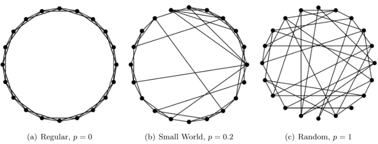
A small-world model is highly connected and transitive (Goldenberg et al., 2010), with a small diameter and large clustering coefficient (2.3). The combination of these two features is not possible with a RGM because as the number of nodes increases the diameter also in-creases, and transitivity is inversely related to the number of nodes (Kolaczyk, 2009). In the development of the small-world model, Watts and Strogatz (1998) envisioned a spectrum of randomness for networks. At one extreme is a regular graph with no randomness. The example regular graph used in this work consists of n nodes equally spaced on the circumference of a circle where each node is connected to the closestk nodes. This implies an edge between node iand the closest k/2 nodes clockwise on the circle andk/2 in the counter-clockwise direction
(a) Regular,p= 0 (b) Small World,p= 0.2 (c) Random,p= 1
Figure 2.1 Demonstration of the Small-World model of Watts and Strogatz (1998). The graphs increase in randomness from right to left.
from node i. An example with n= 20 and k = 4 is shown in the far left plot of Figure 2.1. Regular graphs have a high value of the clustering coefficient, (2.3). At the other end of the randomness spectrum is a random graph. A random graph contains the same number of edges,m=kn, but each edge connects two nodes chosen independently and at random, while excluding the possibility of self-loops and multi-edges. An example of a random graph with n= 20 and m = 4×20 = 80 is shown on the far right of Figure 2.1. Random graphs have a small diameter, i.e., exhibit small-world behavior. The Small-World model, also known as the Watts-Strogatz Model, falls between the regular and random graphs on the randomness spec-trum, while retaining both features of high clustering from a regular graph and the small-world property from a random graph.
The small-world model can also be cast as a generation mechanism and thus classifies as a “pseudo-dynamic” model (Goldenberg et al., 2010). The process of generating a small-world model begins with a regular graph of n nodes and k connections. Each edge is considered in turn and has a fixed, independent probability p of being rewired. If an edge is chosen to be rewired, one end of the edge is relocated to a different node, chosen uniformly from the remaining n−2 nodes. Again, self-loops and multi-edges are disallowed, thus the number of edges remains constant atm=kn. The middle plot of Figure 2.1 shows a small-world network
with probability to rewire, p= 0.2. The parameterp determines the location of the graph on the randomness spectrum. In the extremes,p= 0 implies that no edges are rewired, resulting in the regular graph andp= 1 implies that all edges are rewired, and thus a random graph is simulated.
The disadvantage of a graph produced from the small-world model is that the graph will not have a power law degree distribution. A regular graph has a degenerate degree distribution at degree k, and the degree distribution of a random graph is Binomial. A graph generated from the small-world model will have a degree distribution somewhere between the two extremes; however, because the value of p is often chosen to be small, the degree distribution more often resembles the degenerate distribution of a regular graph. In addition, formal statistical methods do not exist to assess the fit of the model to empirical networks (Goldenberg et al., 2010). Theoretical properties of graphs simulated from the small world model are not easily determined and are described by Kolaczyk (2009) as an “open problem”.
2.2.3 Preferential Attachment
A preferential attachment model is categorized as a “network growth model” (Kolaczyk, 2009) because models of this type are designed to model the evolution of a network over time. The basis of the modern varieties of preferential attachment models was developed by Barab´asi and Albert (1999) specifically to model the expansion of the World Wide Web. The authors were motivated by the observation that new webpages were more likely to form links to the more popular, currently existing pages than the less popular ones. The rationale behind the approach has been referred to as “The rich get richer” or cumulative advantage (Chakrabarti and Faloutsos, 2006) and is related to Zipf’s Law and the Chinese Restaurant Process (Vivar and Banks, 2012).
In contrast to the previously discussed network generating approaches, a preferential at-tachment model allows for the addition of nodes. The process of generating a network begins with n0 nodes and m0 edges. At each iteration one new node is added to the network and
connected toq < n0 existing nodes. The probability a new node connects to an existing nodev
added node will connect to nodev is pv = d(v) X i d(i). (2.4)
Aftertiterations the graph will containn0+tnodes andm0+qtedges. An important property
of graphs produced from the preferential attachment model is a power law degree distribution, i.e., a scale-free graph. As the number of iterations grows, the power law exponentγ in (2.2) approaches 3 (Kolaczyk, 2009) regardless of the number of nodes added at each iteration, q (Chakrabarti and Faloutsos, 2006). The resulting graph also exhibits a small-world behavior. Asymptotic bounds have been determined for the diameter of a preferential attachment graph that relates to the number of nodes logarithmically (Leskovec et al., 2007).
The lack of flexibility of networks generated from the original preferential attachment method has been criticized. First, the graphs may exhibit small-world behavior, but the model does not include a parameter to control it (Vivar and Banks, 2012). Another feature not con-trolled by the model is the power law exponent that always approaches γ = 3. Although the shape of the degree distribution, particularly the tails, may change as new nodes are added, the average degree remains constant atq, while empirical evidence suggests the average degree should increase as the network grows (Chakrabarti and Faloutsos, 2006). The model is un-able to produce networks with a dense core because edges are always added q at a time (Bar et al., 2007), and the method is unable to produce graphs with several connected components or isolated nodes (Chakrabarti and Faloutsos, 2006). Finally, the growth of the diameter as the number of nodes increases does not match reality as recent evidence suggests the diameter actually shrinks as the network grows (Leskovec et al., 2010).
When a deficiency of the original preferential attachment model is presented, it is often followed with a modified version that addresses the stated inadequacy. The simplicity of the original approach (Barab´asi and Albert, 1999) has also contributed to the many existing ex-tensions. Chakrabarti and Faloutsos (2006) detail ten of these extension and the inadequacy of the original preferential attachment model that is addressed. As an example, an initial attractiveness model allows for a more general power law by adding a parameter to the edge
connectivity probability in (2.4) so that it becomes pv = d(v) +A X i [d(i) +A]
with the resulting power law exponentγ(A) = 2 + Aq. The power law is now a function of the parameterA. The forest fire model is an example of a more elaborate variation of the original preferential attachment model (Leskovec et al., 2007). Networks generated from the forest fire model are scale free, have a decreasing diameter, an increasing average degree, are directed, and allows for community structure. Two additional parameters are used in this model: a forward burning probability, pf b, and a backward burning ratio,rbb. At each iteration, a new
node is added to the graph and edges form according to the following steps:
1. Choose an “ambassador node,” w, uniformly at random from the existing nodes of the graph. Form a link between the new node tow.
2. Draw a random number, n1, from the binomial distribution with mean (1−pf b)−1.
3. Choose n of the currently existing edges of node w. Select edges that are directed to node w with probability rbb times less than edges that are directed away from node w.
Letw1, w2, . . . , wn represent the nodes at the other ends of the edges selected.
4. Connect the newly added node with a directed edge tow1, w2, . . . , wn.
5. Repeat steps 2 and 3 recursively for each of thew1, w2, . . . , wn
Extensions to the forest fire method have also been developed to allow for isolated nodes, or orphans, or to choose multiple ambassador nodes.
Preferential attachment models are an example of how many of the algorithmic graph generators are applied to realized networks, and the forest fire model is an example of how complicated the algorithms can become. Simulated networks are mostly used to compare characteristics from a realized network of interest. The goal is for the simulated network to match the realized graph on characteristics studied. Metrics and statistics have also been developed to test the resemblance of the simulated graph to the network of interest. Often
these values relate back to the three main features of a network: power law degree distribution, small diameter, and clustering. Little effort has been made to estimate the parameters of the model given an observed network.
2.3 Graph Analysis: Probabilistic modeling
In contrast to the algorithmic graph generators of the previous section, models described in this section can be described with a likelihood function. Therefore, a statistical model can be constructed for an entire graph with a joint distribution, and statistical inference can be conducted. Controlling parameters can be estimated, the probability of a realized graph can be determined, and the fit of the model can be assessed. It should be noted that although it is possible to generate graphs from models of this type, these models go beyond generation.
Two broad classes of probabilistic modeling of random graphs will be discussed in detail. The first class are exponential random graph models (ERGMs), which specify a joint distri-bution for the collection of edge variables with the goal of describing global network features through interactions of local edge configurations. Conversely, models categorized as latent vari-able models (LVMs) will focus on the interpretation of properties of the individual nodes of the graph (Hunter et al., 2012). This category encompasses a wider range of graph models that are hierarchical in nature. Conditional distributions for edges variables specify the model and are considered to be independent given some latent variable, such as block membership or position within a social space.
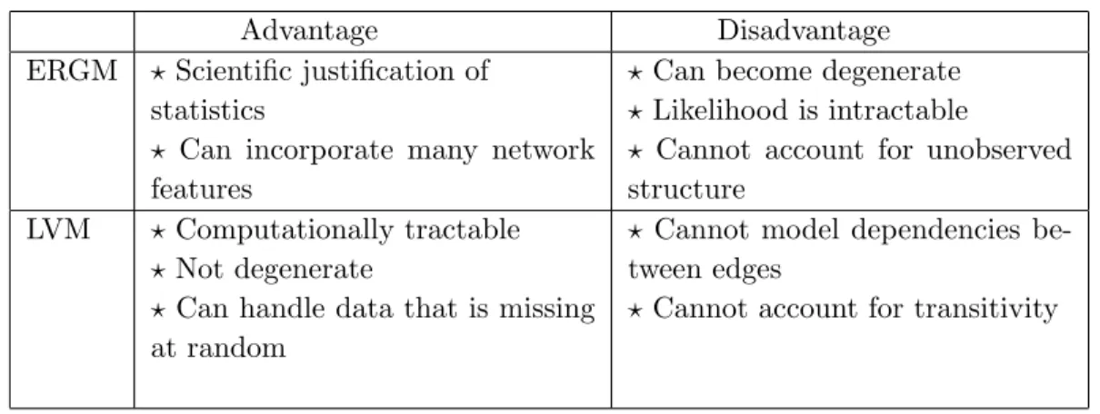
In reference to social networks, Snijders (2007) described ERGMs and a subclass of LVMs, the latent space models, as the two competing models for probabilistic modeling and statistical analysis of networks. Although specific applications may be well-suited for one approach or the other, there are networks where both would be applicable. Each method presents advantages and challenges, a brief summary of which is presented in Table 2.1. Models that integrate the advantages of both approaches while minimizing the difficulties are referred to as “the next generation” of models (Snijders, 2007).
Table 2.1 Comparison of the strengths and weaknesses of the two categories of probabilistic modeling: exponential random graph models (ERGMs) and latent variable models (LVMs).
Advantage Disadvantage
ERGM ? Scientific justification of statistics
? Can incorporate many network features
? Can become degenerate ? Likelihood is intractable
? Cannot account for unobserved structure
LVM ? Computationally tractable ? Not degenerate
? Can handle data that is missing at random
? Cannot model dependencies be-tween edges
? Cannot account for transitivity
2.3.1 Exponential Random Graph Models
The exponential random graph model (ERGM) is a widely-used and extensively-studied class of models under the category of probabilistic modeling. This class arose from collabora-tions between sociology, psychology, and statistics and was originally developed to model social networks. Unlike many of the other analysis techniques discussed, ERGMs have been applied to networks in areas other than that for which it was originally intended (e.g., Groendyke et al., 2012; Simpson et al., 2011). Its popularity can be partially attributed to the model’s ability to represent graph topology while also allowing for complex dependencies.
2.3.1.1 Introduction
An ERGM is specified as a joint distribution for that adjacency matrix, Y, in exponen-tial family form (Kolaczyk, 2009). The exponenexponen-tial family was chosen because the sufficient statistics are explicitly tied to parameters and are equal to their expected values (Holland and Leinhardt, 1981). Let Ω ≡ {y : Pr(Y =y) >0} be the support of the joint distribution. A general functional form of the joint distribution is
Pr(Y=y) = 1 κexp X T⊆C θTgT(y) (2.5) where
• C is the set of all paris of nodes between which an edge could form; most often all pairs of nodes, so|C|= n2
• T ⊆C is a subset of the possible edges, often called a configuration
• θT is a parameter corresponding to configuration T
• gT(y) = Y
(i,j)∈T
yij is a network statistic, which is equal to 1 when configuration T occurs
iny • κ=X Y exp X T⊆C θTgT(y)
is the normalizing constant.
The summation in the exponent of (2.5) is referred to as the negpotential function Q(Y) = X
T⊆C
θTgT(y). (2.6)
Defining the negpotential function (2.6) defines the joint distribution, up to a constant. Speci-fying a particular set of parameters,θT, or equivalently network statistics,gT(y), to be included
in the negpotential specifies an ERGM. Often these statistics are counts of subgraph features, such as the number of edges, number of triangles, or number of edges in a particular block, and the corresponding parameters represent density, transitivity, and block effect, respectively.
Early model development for ERGMs involved the introduction of parameters or statistics to be included in the negpotential function (2.6). Four main phases of ERGM development will be discussed. First, the proposal of a model of form (2.5) for network analysis. Next, the relaxing of an independence assumption to allow for more complex dependence structures, followed by the proposal of parameters not motivated by dependence. The most recent development involves the introduction of parameters designed specifically to address a common issue with the application of an ERGM to realized networks, that of model degeneracy.
Many studies point to the seminal work of Holland and Leinhardt (1981) as the introduction of ERGMs. This work proposed the p1 model, a log-linear model applied to the dyads of a
directed social network. A dyad is defined as a pair of nodes and the possible ties between them, which in an unweighted, directed graph could be 0, 1, or 2. Prior network analysis was descriptive only, focusing on aspects such as the degree distribution or the distribution of nodal
attributes. In contrast, Holland and Leinhardt (1981) were able to stochastically model the patterns of relationships. The p1 model allows for a simultaneous estimation of a parameter
representing reciprocity, or a tendency for a edge to be reciprocated, and a parameter for differential attractiveness, which occurs when a node attracts a comparatively large number of edges. The authors argued both reciprocity and differential attractiveness were common in realized social networks.
Although the p1 model was the first to be able to estimate meaningful parameters, a
disad-vantage is that the dyads are modeled to be independent. This assumption leads to a likelihood that is a product of probabilities for each dyad, which was necessary in order to estimate the parameters with the existing statistical techniques of the time. Relaxing this assumption was identified by Holland and Leinhardt (1981) to be important, yet difficult. The next ERGM development was introduced by Frank and Strauss (1986), who were able to incorporate a more general definition of dependence by adapting methods developed for spatial statistics (Besag, 1974) to social networks. Because of the ability to model a general, complex dependence structure, it is most common for Frank and Strauss (1986) to be cited as the origin of ERGMs. To illustrate the complex dependence structure of a network, Frank and Strauss (1986) in-troduced the dependence graph for social network analysis. Each node in the dependence graph corresponds to a potential edge in the original graph where a connection in the dependence graph indicates the corresponding random variables are conditionally dependent. An important dependence structure is incidence, or Markovian, in which two edges are conditionally depen-dent if they share a common node, and graphs with this dependence structure are referred to as Markov graphs Frank and Strauss (1986). The dependence graph corresponding to a Markov graph does not have edges between disjoint sets of nodes. Stated another way, let {i, j} and {m, n}represent two potential edges in the original, Markov graph and thus two nodes in the dependence graph. If {i, j} ∩ {m, n} = ∅ the two edges are conditionally independent, and there will not be an edge between these nodes in the dependence graph. The set of random variables on which a particular random variable is conditionally dependent, i.e., linked in the dependence graph, will be called its neighborhood. For a Markov graph the neighborhood of edge{i, j} is{{r, s}:{i, j} ∩ {r, s} 6=∅}.
Closely related to the idea of neighborhoods is the Hammersly-Clifford Theorem. This is an important theorem that has been stated and proven in various forms and in multiple references. (For the original see (Clifford, 1990); for one similar to what is used here see (Cressie, 1993, p. 417)) First, assume the network contains a finite numberm of possible edges. Let the support of the joint distribution of Y be designated as Ω and assume there exists ay∗ ∈Ω such the that joint probability distribution is positive, Pr(Y = y∗) > 0. Besag (1974) showed that for y∗ = 0 the negpotential function can be expanded uniquely over Ω as a summation over configurations of random variables, i.e., that the negpotential takes the form shown in (2.6). This result was later generalized for any y∗ ∈Ω (Kaiser and Cressie, 2000). The Hammersly-Clifford Theorem states that the parameter,θT, will be non-zero only if the random variables in
the corresponding configurationT form a clique, where a clique is a single random variable or a set of random variable such that every pair within the set is pairwise mutually conditionally dependent, given the rest of the graph. This theorem implies the dependence structure affects which parameters in (2.6) will be non-zero.
As an example, the non-zero parameters for a Markov graph will correspond to triangles and k-stars. A k-star configuration results fromk edges which all share a common node, with order ranging from k = 1, . . . , n−1. Note that a 1-star is just an edge in the graph. In practice, all order stars are rarely considered because of the large number of parameters this model would include; however, the dependence structure is still incidence. A common model used as an example is the triad model, which consists of a term for 1-stars, i.e., edges, 2-stars, and triangles. The negpotential function of the triad model is
Q(Y) =ρg1(y) +σg2(y) +τ g3(y)
whereρ is a density parameter, σ a parameter for clustering, τ is a parameter that represents transitivity, and the network statistics count the corresponding number of configurations in y (e.g., g2(y) counts the number of 2-stars in the network).
The parameters,θT, included in the negpotential function of a Markov graph are the result of
the incidence dependence structure and the Hammersly-Clifford Theorem. The next refinement in ERGM specification began with Wasserman and Pattison (1996) who proposed parameters
and statistics motivated by the graph topology they represent, rather than the dependence structure. These models were named p∗ in honor of the p1 model (Holland and Leinhardt,
1981), which also included parameters motivated by empirical observation of networks. Four tables of possible parameters are introduced with the p∗ model with a statement that those listed are just a subset of the possibilities.
As an application of the converse of the Hammersly-Clifford theorem, the terms included in the negpotential function of a p∗ model can be used to determine neighborhoods of edges. Thus, a conditional dependence structure is induced by the choice of terms included in the moel. Five methods are suggested for how to choose the parameters of a p∗ model (Wasserman and Pattison, 1996), one of which is to consider the induced conditional dependence between possible edges. Although, even if the conditional dependence is not a modeling consideration, there is still an induced conditional dependence structure. For some example p∗ models, Wasserman and Pattison (1996) describe the induced conditional dependencies, but for others admit that identifying the sets of conditionally dependent edges is not immediate and that some models induce “arbitrary complexity.” Further, varying the parameters in the negpotential can lead to changes in the implied dependence structure. More recently, Goodreau (2007) pared down the list of parameter-choosing methods to two approaches: considering the implied dependence or the combination the of parameters that fit the empirical network best.
The extension to include arbitrary statistics in the negpotential function (2.6) provides a straightforward approach to incorporating exogenous information in an ERGM. The parameters discussed up to this point have been endogenous, or functions of the graph itself (e.g., density or transitivity). Exogenous attributes do not depend on the structure of the graph and can be incorporated at the level of the individual nodes, edges, or as symmetric functions. A main effect term is an example of how to include an exogenous attribute of a node. This parameter varies with the covariate value of the node (Goodreau, 2007). A similar example for pairs of nodes is assortative mixing which attempts to capture the increased probability of edges to form between nodes within the same attribute class (Goodreau et al., 2008). When this effect is uniform across attribute classes, it is referred to as uniform homophily. For example, consider a friendship network between grade-school aged children. A uniform homophily term
Figure 2.2 Configuration of edges which leads to partial conditional dependence.
could represent the higher probability of friendships to form between children within the same grade. Differential homophily allows for a different parameter to describe this effect within the different attribute classes. For the grade-school example, a differential homophily term could be used to describe how friendships are more likely to form between two nodes of the same gender and how females tend to make more friends than males (Hunter et al., 2008b). As a final example, if the covariate is continuous, such as age, the absolute value of the difference can be included as a statistic, and the corresponding parameter would allow the probability to vary monotonically with the value of the absolute difference (Goodreau, 2007). Attribute-based parameters do not affect the dependence structure and thus, including only these parameters leads to a dyad-independence model.
An approach that considers the effect of the dependence structure and higher-order statistics are the two extensions to ERGMs termed “neighborhood-based” models (Pattison and Robins, 2002). The first extension uses “social settings,” or groupings of nodes, typically based on nodal attribute values. Multiple social settings can be defined for a model, and they may be overlapping. Two edges are considered conditionally independent if they do not occupy any common setting, although they are not necessarily conditionally dependent if they do. The purpose of this approach is to limit the number of conditionally dependent random variables, or the size of the neighborhoods. The second extension includes a parameter to account for configurations of at least four nodes such that every pair of edges are part of a path of length three. An example of such a configuration is shown in Figure 2.2. The dependence structure induced by this form of statistics is termed partial conditional dependence. Two random variables are defined to be partially conditionally dependent, if their dependence status is
determined by the state of a third random variable. For the example shown in Figure 2.2, the two dashed, red lines will lie on a path of length three and therefore be conditionally dependent only if the solid, black edge is realized.
Other extensions to the original ERGM that will not be discussed in detail here include an extension to networks with multiple relations (Pattison and Wasserman, 1999), networks with values on the edges (Robins et al., 1999), and including the attributes into the dependence graph to predict node-level attributes given the graph topology (Robins et al., 2001). The final, significant contribution to the development of model parameters for an ERGM to be discussed is the proposal of the alternating or geometrically weighted statistics (Snijders et al., 2006; Robins et al., 2007). Full consideration of this new specifications will be postponed until the section on degeneracy, Section 2.3.1.3, as the terms were developed to combat this specific issue.
Although an ERGM is typically expressed as a joint distribution, it can also be expressed as a conditional log-odds, which allows for a more natural parameter interpretation. Consider the random variable,Yij, representing a potential edge between nodesiandj. The conditional
log-odds forYij implied by the joint specification of an ERGM (2.5) is
logit[Pr(Yij = 1|Yijc =ycij)] = X
T⊆C
θTδg(y)ij (2.7)
where Ycij represents all edges in the network other than edge{i, j} and δg(y)ij is the vector
of change statistics. A chance statistic is
δg(y)ij =gT(y+ij)−gT(yij−)
wheregT(y+ij) is the value of the network statistic if edge{i, j} is present while the rest of the
graph remains unchanged and gT(y−ij) is the analogous value when edge{i, j} is absent. The
change statistic,δg(y)ij, represents the effect on the network statisticgT(y) if random variable
Yij is changed from 0 to 1 and all other random variables remain constant. As an example, if
gT(y) represents the density of the graph, the change statistic is always 1 because the addition
of an edge will always increase the density by 1.
A parameter, θT, of an ERGM is interpreted as the increase in conditional log-odds of a