Working Paper 08-25
Statistics and Econometrics Series 07 May 2008
Departamento de Estadística Universidad Carlos III de Madrid
Calle Madrid, 126 28903 Getafe (Spain) Fax (34) 91 624-98-49
BAYESIAN NON-LINEAR MATCHING OF PAIRWISE MICROARRAY GENE EXPRESSIONS
J.M. Marin1 and C. Nieto2
Abstract
In this paper, we present a Bayesian non-linear model to analyze matching pairs of microarray expression data. This model generalizes, in terms of neural networks, standard linear matching models. As a practical application, we analyze data of patients with Acute Lymphoblastic Leukemia and we find out the best neural net model that relates the expression levels of two types of cytogenetically different samples from them.
Keywords: MCMC computation, microarray data analysis, multidimensional scaling, neural network, spatial Bayesian methods.
1) Departamento de Estadística, Universidad Carlos III de Madrid, e-mail: jmmarin @est-econ.uc3m.es
2) Departamento de Estadística e IO. III, Universidad Complutense de Madrid, e-mail: [email protected]
Bayesian non-linear matching of pairwise microarray gene
expressions
J.M. Marin
1and C. Nieto
2 1: Dep. de Estad´ıstica, U. Carlos III, Getafe 2: Dep. de Estad´ıstica e I.O. III, U. Complutense, MadridAbstract
In this paper, we present a Bayesian non-linear model to analyze matching pairs of microarray expression data. This model generalizes, in terms of neural networks, standard linear matching models. As a practical application, we analyze data of patients with Acute Lymphoblastic Leukemia and we find out the best neural net model that relates the expression levels of two types of cytogenetically different samples from them.
Keywords: MCMC computation, microarray data analysis, multidimensional scaling, neural network, spatial Bayesian methods.
1
Introduction
In Shape and Procrustes Analysis a typical problem is how to match two or more configura-tions of labelled points or landmarks (see Dryden and Mardia (1998)) by applying a geometrical transformation. In Bioinformatics, Green and Mardia (2006) studied the problem of matching two configurations under a linear Bayesian hierarchical model, and Marin and Nieto (2008) derived a generalization of this problem in terms of multiple configurations. In Chemoinfor-matics, Dryden et al. (2007) considered the problem of matching unlabelled point sets under a linear application when two configurations of points were compared, one being treated as a perturbation of the other one.
In this paper, we consider a non-linear model consisting of a linear term plus a neural net-work, between two configurations of points with applications in microarray data analysis. This is a very general approach that enables to consider complex relationships among different levels of expression data. We consider a Bayesian methodology in order to estimate the corresponding parameters of the model.
In Section 2 and Subsection 2.1 we present the problem of matching two configurations by using a non-linear model, under normality, and we derive the posterior distributions of the parameters therein.
In Section 3 we apply previous results in the case of comparing expression levels of a selected group of genes involved in patients with Acute Lymphoblastic Leukemia, based on data derived by Chiaretti et al. (2004).
2
Non-linear relations between configurations of points
Let consider two configurations of n matched points in Rd, x = x
i (i = 1, . . . , n) and y = yi
(i = 1, . . . , n) where one of the configurations is considered fixed, e.g. x, and the other is a random perturbed version of the previous one. If the relation between configurations cannot be expressed in terms of translations or rotations, we can consider a more general non-linear model consisting of a linear model plus a one-layer feed forward neural network,
yij = βj0+λTjxi + M X k=1 βjkΨ(γk0+xTi γk) +εij i = 1, . . . , n j = 1, . . . , d
where, for all i = 1, . . . n, j = 1, . . . , d and k = 1, . . . , M, the parameters of the model are
βj0 ∈R, λj ∈Rd, βjk ∈R, γk0 ∈R and γk ∈Rd. Errorsεij are independently distributed with
a given density fi and Ψ(·) is the activation function that may be a logistic function (see for a
revision Lee (2004)).
In this model each coordinate of point yi is related with each point xi (i = 1, . . . , n) by
means a linear part plus a non linear one in terms of one-hidden layer neural network. Note that the number of hidden nodes, M, may be considered as an unknown parameter.
Alternatively, the model may be expressed in a matrix form as
yi =β00+ ΛxTi +BΨ(γ0+xTi γ) +εi i= 1, . . . , n where β00 d×1 = β10 ... βd0 , Ψ(γ0+xTi γ) M×1 = Ψ(γ10+xTi γ1) ... Ψ(γM0+xTi γM) , B d×M = β11 · · · β1M ... ... ... βd1 · · · βdM , Λ d×d= λ11 · · · λ1d ... ... ... λd1 · · · λdd
2.1
Bayesian inference
In this Section, we shall assume that the number of hidden nodes is known. If normal errors are supposed, the likelihood is
L(β00,Λ, B, γ0, γ, σ2|y)∝ 1 (σ2)nd/2exp ( − 1 2σ2 n X i=1 d X j=1 (yij −βj0−λTjxi− − M X k=1 βjkΨ(γk0+xTiγk))2 ) .
In R2 the model is simplified as L(β00,Λ, B, γ0, γ, σ2|y)∝( 1 σ2) nexp ( − 1 2σ2 " n X i=1 (yi1−β10−λT1xi− − M X k=1 β1kΨ(γk0+xTi γk))2+ n X i=1 (yi2−β20−λT2xi− M X k=1 β2kΨ(γk0 +xTi γk))2 #) .
In order to carry out Bayesian inference, we must first introduce the prior distributions for the parameters of the model assuming a relatively diffuse prior distribution structure.
Let assume that the prior distribution ofσ2 is inverted-gamma IG(α, β), then the posterior
distribution of σ2 is p(σ2 |y,· · ·)∝(σ2)−(α+1)exp ½ −β σ2 ¾ ·( 1 σ2) nexp ( − 1 2σ2 " n X i=1 (yi1−β10−λT1xi− − M X k=1 β1kΨ(γk0+xTi γk))2 + n X i=1 (yi2−β20−λT2xi− M X k=1 β2kΨ(γk0+xTi γk))2 #) ∝ (σ2)−(α+1+n)exp ½ − 1 σ2 (β+A) ¾ , where A = 1 2 " n X i=1 (yi1−β10−λT1xi − M X k=1 β1kΨ(γk0+xTiγk))2 + n X i=1 (yi2−β20−λT2xi− M X k=1 β2kΨ(γk0 +xTi γk))2 # .
Hence, the posterior distribution is also inverted gamma, σ2 |y,· · · ∼IG(α+n, β +A).
Let assume that prior distributions ofβj0 ∼N(µβj0, σ
2
βj0), withj = 1,2.Then, the posterior
distribution is βj0 |y,· · · ∼N( Dj0 2Cj0 , C−1 j0 ) where Cj0 = σ21 βj0 + n σ2; Dj0 = 2µβj0 σ2 βj0 +2 n P i=1Rij0 σ2 ; Rij0 =yij−λTjxi − M X k=1 βjkΨ(γk0+xTi γk).
Let assume that the prior distribution ofλrs, forr = 1,2 ands= 1,2 isλrs∼N(µλrs, σλ2rs);
then, the posterior distribution is
λrs |y,· · · ∼N( Drs C , C
−1
where Crs= n P i=1 x2 is σ2 +σ21 λrs; Drs = n P i=1 Mirsxis σ2 + µλrs σ2 λrs; Mirs =yir−βr0−λrsxis− M X k=1 βrkΨ(γk0+xTi γk).
Let assume, for j = 1,2 and s = 1, . . . , M, that the prior distribution of βjs, is βjs ∼ N(µβjs, σ2βjs); then, the posterior distribution is
βjs|y,· · · ∼N( Dj Cj , C−1 j ) where Cj = n P i=1 Ψ2(γ s0+xTi γs) σ2 + 1 σ2 βjs ; Dj = n P i=1 RijΨ(γs0+xTi γs) σ2 + µβjs σ2 βjs ; Rij = yij −βj0−λTjxi − M X k=1 k6=s βjkΨ(γk0+xTi γk).
Let assume that the prior distribution of γrs, for r = 1, . . . , M and s = 0,1,2 is γrs ∼ N(µγrs, σγ2rs); then, the posterior distribution is
p(γrs|y,· · ·)∝exp − 1 2σ2 n X i=1 (yi1−β10−λT1xi− M X k=1 k6=r β1kΨ(γk0+xTi γk)− −β1rΨ(γr0 +xTi γr))2+ n X i=1 (yi2−β20−λT2xi − − M X k=1 k6=r β2rΨ(γk0+xTiγk)−β2rΨ(γr0+xTi γr))2 ·exp ½ − 1 2σ2 γrs (γ2 rs−2µγrsγrs) ¾ ∝exp ½ − 1 2σ2 γrs (γrs2 −2µγrsγrs) ¾ ·exp ( − 1 2σ2 " n X i=1 (Ri1−β1rΨ(γr0+xTi γr))2+ exp ( − 1 2σ2 " n X i=1 (Ri1−β1rΨ(γr0+xTi γr))2+ n X i=1 (Ri2−β2rΨ(γr0+xTiγr))2 #) ,
where, for all i= 1, . . . , nand j = 1,2, Rij =yij −βj0−λTjxi− M X k=1 k6=r βjkΨ(γk0+xTi γk).
Given these conditional distributions, we can apply an MCMC algorithm to simulate a sam-ple from the joint posterior distribution. All conditional distributions are normal and inverted gamma, except that of parameter γ. Hence, we can introduce a Metropolis-Hasting step, inside a Gibbs sampling algorithm, with a normal as proposal distribution. As an alternative to stan-dard Gibbs sampling, Wong and Liang (1997) proposed a simulated tempering with dynamic weighting (STWD) algorithm to deal with training of neural networks.
The size of the neural net, namely, the number of hidden nodes M can be considered as a parameter. In this case, it may be applied a reversible jump methodology to explore among spaces of different dimension (see e.g. Muller and Rios-Insua (1998) and Andrieu et al. (2001)). Nevertheless, in complex models like neural nets, problems of identifiability may appear and other methods may be considered (see Titterington (2004) for a revision). As a measure of complexity and fit of models, we have used a modified version of a DIC coefficient as pointed out by Richardson (2002), and Celeux et al. (2006) who labeled this version as DIC3. This
criterion is well adapted to the case of neural networks with different possible architecture. The expression of this coefficient is
DIC3 =−4Eθ|y[logf(y|θ)] + 2 log ˆf(y),
where ˆf(y) = Qn
i=1
ˆ
f(yi), and ˆf(yi) = Eθ|y[f(yi |θ)].
3
Application in microarray data expressions of
Lym-phoblastic Leukemia
We have chosen a microarray experiment, depicted in the databaseALLfrom the BioConductor bundle (see Gentleman et al. (2004b)), originally rendered by Chiaretti et al. (2004). We have taken a subset of 79 samples representing patients with B-cell acute lymphoblastic leukemia, and we have considered, first, the samples with BCR/ABL fusion gene (37 patients) and then, the cytogenetically normal samples (42 patients).
We sought a group of genes with different expression levels in above samples. For that, we have used the genefilter package of the BioConductor bundle (Gentleman et al. (2004) and Gentleman et al. (2004b)) and we have selected 2391 probesets from the original 12625 ones for our analysis, deleting those with no expression or low variability across all samples. Then, by using the multtest package, we have considered the criterion provided by the false discovery rate (FDR), that is, the expected proportion of false positives among the genes that are significant. We have used the procedure of Benjamin and Hochberg (1995) to control the FDR at a level of 0.05. After this procedure, we have obtained 102 significantly different expressed genes.
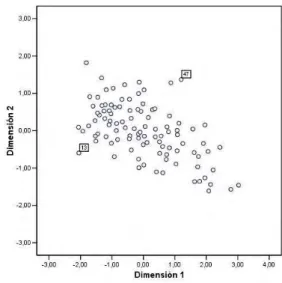
As a previous step we have projected the selected genes in a two-dimensional map in order to determine which function relates them. For that, we have computed the Euclidean distances
between pairs of genes in each group and we have built a map by using an INDSCAL Analysis (see for references therein e.g. Borg and Groenen (2005) and Marin and Nieto (2008)). In order to program the INDSCAL Analysis we have used softwareSASv. 9.1 running in a Pentium IV, 3.2 Ghz. processor.
In figures 1 and 2 we show the positions of genes in the two groups of patients, after applying the INDSCALAnalysis. In these figures, numbers identify two specific genes in order to visualize their situation in the space. We will consider the cytogenetically normal group as the fixed configuration of points.
Figure 1: Group cytogenetically normal Figure 2: Group with the BCR/ABL fu-sion
In order to program model 2.1 we have used as software WinBugs (see Lunn et al. (2000)) running in a Pentium IV, 3.2 Ghz. processor. We have used, as prior distributions ofβ00,Λ, B, γ0
and γ, normal distributions with zero means and high variances. For parameter σ2 we have
used a prior inverted gamma distribution with high variance also. All programs are disposable by request to the corresponding author.
In table 1 we show DIC3 values for different number of hidden nodes M, after a total of
100000 iterations with 50000 iterations for burn-in. Lowest value is obtained for M = 1.
M 1 2 3 4 DIC3 -1494.565 -1493.17 -1492.177 -1488.328 M 5 6 7 8 DIC3 -1486.23 -1486.049 -1484.409 -1484.714 M 9 10 DIC3 -1483.864 -1481.183
Table 1: DIC3 values vs number of hidden nodes M
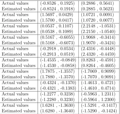
We derive the posterior distributions of the parameters of the M = 1 model. We test the results by dividing the sample of 102 genes, in a random training set with 80% of observations
and a test set with the resting ones. We considered a total of 600000 iterations, with 300000 iterations for burn-in, and three different chains with random initialization points. Post hoc
analysis of chains showed that there were not a significant departure from convergence. Results of predictions and actual values of the validation set are in table 2, showing that predictions are accurate. Actual values (-0.8526 , 0.1925) (0.2886 , 0.5641) Estimated values (-0.8524 , 0.1918) (0.2885 , 0.5623) Actual values (1.5697 , 0.0429) (1.0721 , 0.0091) Estimated values (1.5700 , 0.0417) (1.0720 , 0.0077) Actual values (0.0537 , 0.1107) (2.2148 , -1.0531) Estimated values (0.0538 , 0.1089) (2.2150 , -1.0540) Actual values (0.5167 , -0.6055) (1.9068 , -0.3414) Estimated values (0.5168 , -0.6073) (1.9070 , -0.3424) Actual values (-0.2918 , 0.0534) (2.4316 , -0.4448) Estimated values (-0.2913 , 0.0519) (2.4320 , -0.4459) Actual values (-1.4535 , -0.0849) (0.8263 , -0.4591) Estimated values (-1.4530 , -0.0858) (0.8264 , -0.4605) Actual values (1.7875 , -1.3557) (-1.7069 , 0.9099) Estimated values (1.7880 , -1.3570) (-1.7070 , 0.9091) Actual values (-0.4324 , -0.1370) (-1.4613 , 0.4721) Estimated values (-0.4321 , -0.1383) (-1.4610 , 0.4714) Actual values (-1.2277 , 0.3238) (-0.5963 , 1.2311) Estimated values (-1.2280 , 0.3230) (-0.5964 , 1.2300) Actual values (1.6281 , -1.3630) (-1.5291 , -0.1417) Estimated values (1.6280 , -1.3640) (-1.5290 , -0.1424)
Table 2: Predictions and actual values of validation set
4
Discussion and future developments
The proposed model can be useful to relate different expression levels in two microarrays, corresponding to different conditions in a group of genes. Moreover, this model can be useful to find relations among expressions, by selecting some critical genes, or to assess diagnostic forecasting by comparing positions of genes in different times of a given illness.
One possible generalization may be to consider multiple comparisons among more than two microarrays. As a technical issue, in order to deal with non-linear matching problems, it may be interesting to introduce the class of Gaussian Processes that generalize neural nets models.
References
Andrieu, C., de Freitas, N. and Doucet, A. (2001). Robust Full Bayesian Learning for Radial Basis Networks. Neural Computation 13(10), 2359–2407.
Benjamini, Y. and Hochberg, Y. (1995). Controlling the false discovery rate: a practical and powerful approach to multiple testing. Journal of the Royal Statistical Society, Series B,57, 289–300.
Borg, I. and Groenen, P. J. F. (2005). Modern Multidimensional Scaling. Springer, New York. Celeux, G., Forbes, F., Robert, C. P. and Titterington, D. M. (2006). Deviance Information
Criteria for Missing Data Models. Bayesian Analysis 1(4), 651–674.
Chiaretti, V., Li, X., Gentleman, R., Vitale, A., Vignetti, M., Mandelli, F., Ritz, J. and Foa, R. (2004). Gene expression profile of adult T-cell acute lymphocytic leukemia identifies distinct subsets of patients with different response to therapy and survival.Blood,103(7), 2771–2778. Dryden, I. L., Hirst, J. D. and Melville,J.L. (2007). Statistical analysis of unlabelled point sets:
comparing molecules in chemoinformatics. it Biometrics 63(1), 237–251.
Dryden, I. L. and Mardia, K. V. (1998). Statistical shape analysis. Wiley, Chichester.
Gentleman, R., Carey, V., Huber, W., Irizarry, R. and Dudoit, S. (Eds.) (2004). Bioinformatics and Computational Biology Solutions Using R and Bioconductor. Springer, New York. Gentleman, R., Carey, V., Bates, D., Bolstad, B., Dettling, M., Dudoit, S., Ellis, B., Gautier,
L., Ge, Y., Gentry, J., Hornik, K., Hothorn, T., Huber, W., Iacus, S., Irizarryand, R., Leisch, F., Li, C., Maechler, M., Rossiniand, A., Sawitzki, G., Smith, C., Smyth, G., Tierneyand, L., Yang, J. and Zhang, J. (2004b). Bioconductor: Open software development for computational biology and bioinformatics. Genome Biology 5, R80. url = http://www.bioconductor.org Green, P. J. and Mardia, K. V. (2006). Bayesian alignment using hierarchical models with
applications in protein Bioinformatics. Biometrika 93(2), 235–254.
Lee, H. K. H. (2004). Bayesian nonparametrics via neural networks. Asa-Siam, Philadelphia. Lunn, D. J., Thomas, A., Best, N. and Spiegelhalter, D. (2000). WinBUGS – a Bayesian
modelling framework: concepts, structure, and extensibility. Statistics and Computing 10
325–337.
Marin, J. M. and Nieto, C. (2008). Spatial Matching of Multiple Configuratios of Points with a Bioinformatics Application. Comm. in Stat. T. and Meth. 37, 1977–1995.
Muller, P. and Rios-Insua, D. (1998). Issues in Bayesian Analysis of Neural Network Models.
Neural Computation 10(3), 749–770.
Richardson, S. (2002). Discussion of Spiegelhalter et al.Journal of the Royal Statistical Society, Series B631.
Titterington, D. M. (2004). Bayesian Methods for Neural Networks and Related Models. Sta-tistical Science 19(1), 128–139.
Wong, W. H. and Liang, F. M. (1997). Dynamic weighting in Monte Carlo and optimization.