with Modern GPU Technology
Reza Amouzgar
Thesis submitted for the degree of
Doctor of Philosophy
Newcastle University
Faculty of Science, Agriculture and Engineering
School of Civil Engineering and Geosciences
i
Earthquake-induced tsunamis commonly propagate in the deep ocean as long waves and develop into sharp-fronted surges moving rapidly coastward, which may be effectively simulated by hydrodynamic models solving the nonlinear shallow water equations (SWEs). Tsunamis can cause substantial economic and human losses, which could be mitigated through early warning systems given efficient and accurate modelling. Most existing tsunami models require long simulation times for real-world applications. This thesis presents a graphics processing unit (GPU) accelerated finite volume hydrodynamic model using the compute unified device architecture (CUDA) for computationally efficient tsunami simulations. Compared with a standard PC, the model is able to reduce run-time by a factor of > 40. The validated model is used to reproduce the 2011 Japan tsunami. Two source models were tested, one based on tsunami waveform inversion and another using deep-ocean tsunameters. Vertical sea surface displacement is computed by the Okada model, assuming instantaneous sea-floor deformation. Both source models can reproduce the wave propagation at offshore and nearshore gauges, but the tsunameter-based model better simulates the first wave amplitude. Effects of grid resolutions between 450-3600 m, slope limiters, and numerical accuracy are also investigated for the simulation of the 2011 Japan tsunami. Grid resolutions of 1-2 km perform well with a proper limiter; the Sweby limiter is optimal for coarser resolutions, recovers wave peaks better than minmod, and is more numerically stable than Superbee. One hour of tsunami propagation can be predicted in <1 minute using 1350 m or coarser resolutions. Run-time is reduced by >50 times on a regular low-cost PC-hosted GPU, compared to a single CPU. For 450 m resolution on a larger-memory server-hosted GPU, performance increased by ~70 times. Finally, two adaptive mesh refinement (AMR) techniques including simplified dynamic adaptive grids on CPU and a static adaptive grid on GPU are introduced to provide multi-scale simulations. Both can reduce run-time by ~3 times while maintaining acceptable accuracy. The proposed computationally-efficient tsunami model is expected to provide a new practical tool for tsunami modelling for different purposes, including real-time warning, evacuation planning, risk management and city planning.
iii
I would like to express my deepest gratitude to my supervisors, Prof. Qiuhua Liang and Prof. Peter Clarke, for their patience, invaluable advice, constructive comments, guidance, and encouragements. My supervisors have enabled me to fulfil this thesis and it has been my honour to be their student. When I was searching for a PhD project I was very delighted when I realised Prof. Liang’s research is about computational hydraulics at Newcastle University and part of his active research and interest is related to natural hazards which was exactly what I was looking for. Among the available research program I have been always keen to study tsunami modelling and contribute in this field of knowledge so if I can be of any help for those people around the world who might be vulnerable to this disastrous event.
I would also like to thank Dr Stephen McGough (Durham University) and Dr William Blewitt (Newcastle University) from school of computing sciences for their seminar and talks about high-performance computing.
After model development I had the opportunity to visit the disaster prevention institute (DPRI), Kyoto University of Japan to undertake the preliminary 2011 Tohoku tsunami modelling. In this regard I would like to give special thanks to Dr Tomohiro Yasuda and Prof. Hajime Mase for their valuable assistance providing necessary data and information during my academic visit. I would also like to extend my thanks to peers, colleagues, and researchers who I met during my work so I could ask my questions, discuss and share our views including Hongbin Zhang, Xilin Xia, Jingming Hou, Jingchun Wang, Luke Smith, and Ciprian Spatar. My thanks also go to the administrative staff in School of Civil Engineering and Geosciences, SAgE Faculty workshop organisers, librarians and computing technicians for the services they provided especially Melissa Ware, Hannah Lynn, Graham Patterson and Iain Woodfine.
Finally I would like to express my sincere gratitude to my parents for their continued love and support, I owe my achievements to them. Without their continuous help and support I could not be able to start and continue for my post graduate studies in overseas.
v
1D One-dimensional
2D Two-dimensional
3D Three-dimensional
AMR Adaptive Mesh Refinement API Application Processing Interface CFL Courant-Friedrichs-Lewy
COMCOT Cornell Multi-grid Coupled Tsunami Model
COULWAVE Cornell University Long and Intermediate Wave Modelling Package CPU Central Processing Unit
CUDA Compute Unified Device Architecture
DART Deep-ocean Assessment and Reporting of Tsunamis DCRC Disaster Control Research Centre
DG Discontinuous Galerkin
DP Double Precision
DPRI Disaster Prevention Research Institute, Kyoto University, Japan DRAM Dynamic Random Access Memory
FDM Finite Difference Method FEM Finite Element Method
FUNWAVE Fully Nonlinear Boussinesq model FVM Finite Volume Method
GEONET GPS Earth Observation Network
vi GPS Global Positioning System GPU Graphics Processing Units HLL Harten, Lax, van Leer
HLLC Harten, Lax, van Leer-Contact HPC High-Performance Computing JMA Japan Meteorological Agency LES Large Eddy Simulation
LSWE Linear Shallow Water Equations MOST Method of Splitting Tsunami MPI Message Passing Interface
MUSCL Monotonic Upstream-Centered Scheme for Conservation Laws NLB Non-Linear Boussinesq model
NLSWE Non-linear Shallow Water Equations
NOAA National Oceanic and Atmospheric Administration NVIDIA An American global Technology Company
OBP Ocean Bottom Pressure Gauges ODE Ordinary Differential Equation OpenCL Open Computing Language OpenMP Open Multiple Processing PC Personal Computer POM Princeton Ocean Model RAM Random Access Memory
vii SFC Sierpinski space filling curves SMF Submarine Mass Failure SP Single Precision
SPH Smooth Particle Hydrodynamics STL Standard Template Library SWE Shallow Water Equations
TIME Tsunami Inundation Modeling Exchange
TsunAWI Alfred Wegener Institute for polar and marine research
TUNAMI Tohoku University’s Numerical Analysis Model for Investigation of tsunamis TVD Total Variation Diminishing
UCSB University of California, Santa Barbara UN United Nations
USGS United States Geological Survey VOF Volume of Fluid
ix
Abstract ... i
Acknowledgments ... iii
Abbreviations ... v
List of Figures ... xiii
List of Tables ... xix
Chapter 1 Introduction 1
1.1 Introduction and motivation of the research ... 1
1.1.1 Tsunami effects and tsunami modelling... 1
1.1.2 Brief history of numerical tsunami modelling ... 3
1.2 Tsunami source model ... 5
1.3 High-performance computing ... 5
1.4 Aim and objectives ... 7
1.5 Thesis outline ... 7
Chapter 2 Literature Review 9
2.1 Tsunami models and numerical schemes ... 9
2.2 Acceleration techniques for tsunami simulations ... 20
2.2.1 Mathematical models ... 21
2.2.2 Adaptive grid techniques ... 24
2.2.3 High-performance computing ... 26
2.3 Review of parallel shallow flow models ... 27
2.4 Source models ... 34
2.5 Review of 2011 Japan tsunami simulations ... 38
2.6 Summary ... 45
Chapter 3 Finite Volume Godunov Type Tsunami Model 47
3.1 Governing equations and numerical scheme ... 47
x
3.1.3 Second order accuracy in space and time ... 55
3.1.4 Boundary conditions ... 56
3.1.5 Stability criterion ... 58
3.2 Parallel computing ... 58
3.3 OpenMP parallel computing on CPU ... 59
3.4 GPU parallel computing and CUDA implementation ... 60
3.4.1 Domain structure ... 62
3.4.2 Kernel structure ... 64
3.4.3 Time-step reduction ... 65
3.4.4 Floating point precision effects ... 65
3.4.5 Model structure ... 66
3.5 Summary ... 67
Chapter 4 Model Validation and Performance 69
4.1 Test cases ... 69
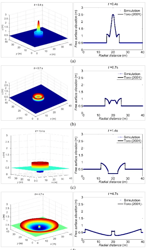
4.1.1 Circular dam-break ... 70
4.1.2 Dam-break wave interacting with three humps ... 72
4.1.3 2D run-up of a solitary wave on a conical island ... 76
4.1.4 Laboratory-Scale Monai Tsunami Benchmark Test ... 83
4.1.5 Hokkaido Nansei-Oki tsunami ... 87
4.2 Summary ... 91
Chapter 5 Case Study of Tohoku Japan Tsunami, 2011 93
5.1 Introduction ... 93
5.2 Research area ... 94
5.3 Tsunami generation and model initialization ... 95
5.3.1 Fault parameters by tsunami waveform inversion ... 98
5.3.2 Fault parameters from tsunameter measurements ... 100
xi
5.4.2 Model-observation comparison ... 103
5.4.3 Evaluation of the source models ... 108
5.4.4 Effect of spatial resolution and the choice of slope limiter ... 111
5.5 Potential sources of errors in tsunami simulation ... 137
5.6 The computational time of tsunami waves ... 139
5.7 Summary ... 140
Chapter 6 Adaptive Grid Technologies for Tsunami Modelling 143
6.1 Introduction ... 143
6.2 Dynamic adaptive grid ... 144
6.2.1 Grid generation and neighbour identification ... 144
6.2.2 Grid adaptation indicator ... 145
6.2.3 Dynamic grid adaptation ... 147
6.2.4 Conservative flux calculation and flow information on newly created cells ... 147
6.2.5 Test case – reconsideration of the Monai tsunami benchmark test ... 148
6.3 Dynamic adaptive grid on GPU ... 149
6.4 Static mesh refinement on GPU ... 152
6.4.1 Model validation – reconsideration of conical island tsunami benchmark ... 154
6.4.2 Model validation – reconsideration of the Japan 2011 tsunami ... 156
6.5 Summary ... 158
Chapter 7 Conclusions and Future Work 161
7.1 Conclusions ... 161
7.1.1 Hydrodynamic modelling of tsunamis using GPU technology ... 161
7.1.2 Simulation of the 2011 Japan tsunami ... 162
7.1.3 Adaptive mesh refinement (AMR) techniques ... 163
7.2 Future work and recommendations ... 164
7.2.1 Hydrodynamic model ... 164
xii
7.2.4 Parallelization ... 168
xiii
Figure 2.1 Schematic view of linear wave characteristics... 9
Figure 2.2 Adaptive grid techniques diagram for tsunami simulations. ... 25
Figure 2.3 Parallel computing techniques for tsunami simulations. ... 34
Figure 2.4 Diagram for tsunami simulation from generation to inundation. ... 38
Figure 2.5 The Sanriku coast in Tohoku region, is located between 38.5̊ N and 40̊ N (Maeda et al., 2011). Ocean bottom pressure gauges (OBP) called TM1 and TM2 off Kamaishi, Northern Japan, shown with triangles. ... 41
Figure 3.1 Sketch of the bathymetry/topography and free surface elevation. ... 48
Figure 3.2 Well-balanced scheme for dry-bed applications. ... 50
Figure 3.3 The solution structure of the HLLC approximate Riemann solver. ... 52
Figure 3.4 Computational cells inside and outside the boundary. ... 57
Figure 3.5 Parallel system with shared memory. ... 59
Figure 3.6 Core comparison between a CPU and a GPU. ... 61
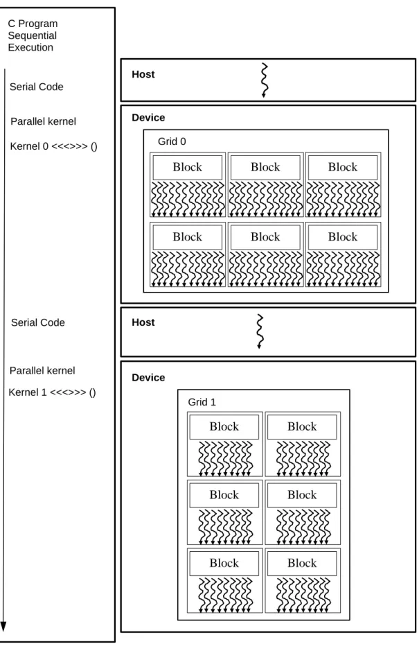
Figure 3.7 Heterogeneous parallel programming diagram. ... 62
Figure 3.8 Heterogeneous parallel programming structure. ... 63
Figure 3.9 Transferring 2D array to 1D. ... 64
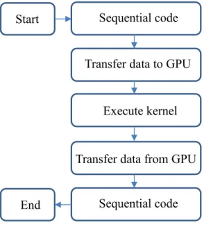
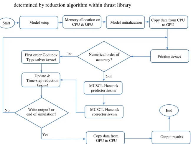
Figure 3.10 Flowchart of the GPU hydrodynamic tsunami model. ... 67
Figure 4.1 Hardware devices used for the simulations: (a) CPU Intel Core i5-2500; (b) GPU GTX 560 Ti; (c) Tesla M2075 GPU on a server. ... 69
Figure 4.2 Circular dam-break: left column: 3D water surfaces, right column: corresponding central water surface profiles at (a) t = 0.4 s; (b) t = 0.7 s; (c) t = 1.4 s; (d) t = 4.7 s... 71
Figure 4.3 Dam-break over three humps: initial conditions and bed topography. ... 72
Figure 4.4 Dam-break over three humps: 3D water surface elevation at (a) t = 2 s; (b) t = 6 s; (c) t = 12 s; (d) t = 30 s; (e) t = 60 s; (f) t = 300 s. ... 73
Figure 4.5 Dam break over three humps: water depth histories predicted by the 2nd-order numerical scheme at different resolutions at the three gauge points, (a) P1; (b) P2; (c) P3. ... 74
Figure 4.6 Dam break over three humps: water depth histories predicted by the 1st and 2nd-order accurate numerical schemes at the 0.1m spatial resolution at the three gauge points, (a) P1; (b) P2; (c) P3. ... 75
Figure 4.7 Dam break over three humps: GPU speedup against the number of cells being used for simulations. ... 76
Figure 4.8 Solitary wave run up on a conical island: computational domain, boundary conditions and gauge locations. ... 77
xiv
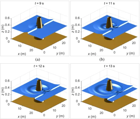
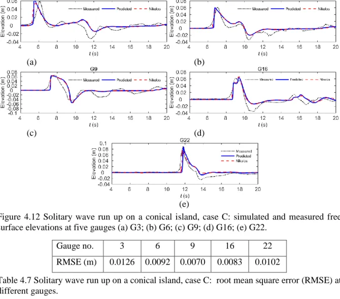
different output times (a) t = 9 s; (b) t = 12 s; (c) t = 13 s; (d) t = 14 s. ... 78 Figure 4.10 Solitary wave run up on a conical island, case B: simulated and measured free surface elevations at five gauges (a) G3; (b) G6; (c) G9; (d) G16; (e) G22. ... 79 Figure 4.11 Solitary wave run up on a conical island, case C: 3D view of the wave run up at time (a) t = 9 s; (b) t = 11 s; (c) t = 12 s; (d) t = 13 s. ... 80 Figure 4.12 Solitary wave run up on a conical island, case C: simulated and measured free surface elevations at five gauges (a) G3; (b) G6; (c) G9; (d) G16; (e) G22. ... 81 Figure 4.13 Solitary wave run up on a conical island, case C: effect of grid resolution. ... 82 Figure 4.14 Monai tsunami benchmark: (a) problem domain, (b) incident tsunami wave. ... 83 Figure 4.15 Monai tsunami benchmark: three-dimensional view of free surface elevation at time (a) t = 12 s; (b) t = 14 s; (c) t=16 s; (d) t=17 s; (e) t=18 s; (f) t=20 s. ... 85 Figure 4.16 Monai tsunami benchmark: 1st and 2nd-order prediction of free surface elevation at three gauges, in comparison with laboratory measurements, at gauges (a) G5; (b) G7; (c) G9. ... 86 Figure 4.17 Hokkaido Nansei-Oki tsunami: computational domain and initial water level. ... 87 Figure 4.18 Hokkaido Nansei-Oki tsunami: (a) 3D view of original bathymetry/topography (b) 3D view of bathymetry/topography with extended cells/layers. ... 88 Figure 4.19 Hokkaido Nansei-Oki tsunami: 2D view of wave propagation at (a) t = 300 s with original boundary; (b) t = 500 s with original boundary; (c) t = 300 s with extended cells/layers at boundaries; (d) t = 500 s with extended layers at boundaries. ... 89 Figure 4.20 Hokkaido Nansei-Oki tsunami: 3D view of tsunami wave propagation at time (a) t = 0 s; (b) t = 100 s; (c) t = 300 s; (d) t = 500 s, (e) t = 2400 s. ... 90 Figure 4.21 Hokkaido Nansei-Oki tsunami: time histories of water surface level predicted with the first and second-order accurate models, compared the measurements at Esashi tide gauge. ... 91 Figure 5.1 Epicentre of the 11 March 2011 Japan earthquake (orange star) reported by USGS. Also shown are the locations of deep-ocean tsunameters, nearshore GPS buoys, and wave gauges (Wei et al., 2013). ... 94 Figure 5.2: Computational domain for the 2011 Japan tsunami and locations of gauges where the green filled circles represent the GPS buoys, dark blue squares the wave gauges, red filled diamonds the pressure gauges, and the yellow filled triangle the deep-ocean tsunameter. The red star represents the epicentre reported by USGS. ... 95 Figure 5.3: Okada model: (a) fault plane as shown in red; (b) fault geometry (c) projection of fault on earth surface (Wang, 2009)... 97 Figure 5.4: Slip distributions predicted by tsunami waveform inversion by (Fujii et al., 2011). The order of numbering of the 40 subfaults can be inferred from the numbered subfaults in the northernmost and southernmost. ... 98
xv
earthquake computed by Okada’s solution (‘source 1’). The fault parameters and information are estimated by tsunami waveform inversion as provided by Fujii et al. (2011). The red star indicates the epicentre provided by the USGS. ... 100 Figure 5.6: Tsunami source from tsunameter measurements for the 2011Japan tsunami. The orange area in the plots for stations D21418 and D21401 shows the interval of the time series used in the inversion. The star indicates the epicentre reported by USGS. The purple lines are the plate boundaries. The black boxes represent the tsunami unit sources precomputed in NCTR’S database. The numbers in boxes indicate the sources number in Table 5.3 (Wei et al., 2014). ... 101 Figure 5.7: Instantaneous seafloor (and hence water level) deformation of the 2011 Tohoku earthquake computed by the Okada model (‘source 2’). The tsunami source inferred from measurements of tsunameter measurements in deep-ocean is provided by Wei et al. (2014). ... 102 Figure 5.8: Evolution of tsunami wave based on the initial conditions provided by ‘source 1’ at different times: (a) t = 10 min; (b) t = 20 min; (c) t = 30 min; (d) t = 35 min; (e) t = 40 min; (f) t = 50 min; (g) t = 60 min; (h) t = 70 min; (i) t = 80 min. ... 104 Figure 5.9: Evolution of tsunami wave based on the initial conditions provided by ‘source 2’ at different times: (a) t = 10 min; (b) t = 20 min; (c) t = 30 min; (d) t = 35 min; (e) t = 40 min; (f) t = 50 min; (g) t = 60 min; (h) t = 70 min; (i) t = 80 min. ... 105 Figure 5.10: Model-observation comparison at 6 GPS buoys with two different source models. ... 109 Figure 5.11: Model-observation comparison at 6 coast gauges with different two source models. ... 109 Figure 5.12: Model-observation comparison at two bottom pressure gauges with two different source models. ... 110 Figure 5.13: Model-observation comparison at DART buoy 21418 with two different source models. ... 110 Figure 5.14: The sensitivity analysis results considering different resolutions and slope limiters for ‘source 1’ at gauge 807, a) first-order accuracy b) minmod limiter c) sweby limiter d) superbee limiter. ... 113 Figure 5.15: The sensitivity analysis results considering different resolutions and slope limiters for ‘source 1’ at gauge 804, a) first-order accuracy b) minmod limiter c) sweby limiter d) superbee limiter. ... 114 Figure 5.16: The sensitivity analysis results considering different resolutions and slope limiters for ‘source 1’ at gauge 802, a) first-order accuracy b) minmod limiter c) sweby limiter d) superbee limiter. ... 115 Figure 5.17: The sensitivity analysis results considering different resolutions and slope limiters for ‘source 1’ at gauge 803, a) first-order accuracy b) minmod limiter c) sweby limiter d) superbee limiter. ... 116
xvi
for ‘source 1’ at gauge 801, a) first-order accuracy b) minmod limiter c) sweby limiter d) superbee limiter. ... 117 Figure 5.19: The sensitivity analysis results considering different resolutions and slope limiters for ‘source 1’ at gauge 806, a) first-order accuracy b) minmod limiter c) sweby limiter d) superbee limiter. ... 118 Figure 5.20: The sensitivity analysis results considering different resolutions and slope limiters for ‘source 1’ at gauge 613, a) first-order accuracy b) minmod limiter c) sweby limiter d) superbee limiter. ... 119 Figure 5.21: The sensitivity analysis results considering different resolutions and slope limiters for ‘source 1’ at gauge 602, a) first-order accuracy b) minmod limiter c) sweby limiter d) superbee limiter. ... 120 Figure 5.22: The sensitivity analysis results considering different resolutions and slope limiters for ‘source 1’ at gauge 202, a) first-order accuracy b) minmod limiter c) sweby limiter d) superbee limiter. ... 121 Figure 5.23: The sensitivity analysis results considering different resolutions and slope limiters for ‘source 1’ at gauge TM-1, a) first-order accuracy b) minmod limiter c) sweby limiter d) superbee limiter. ... 122 Figure 5.24: The sensitivity analysis results considering different resolutions and slope limiters for ‘source 1’ at gauge D21418, a) first-order accuracy b) minmod limiter c) sweby limiter d) superbee limiter. ... 123 Figure 5.25: The sensitivity analysis results considering different resolutions and slope limiters for ‘source 2’ at gauge 807, a) first-order accuracy b) minmod limiter c) sweby limiter d) superbee limiter. ... 124 Figure 5.26: The sensitivity analysis results considering different resolutions and slope limiters for ‘source 2’ at gauge 804, a) first-order accuracy b) minmod limiter c) sweby limiter d) superbee limiter. ... 125 Figure 5.27: The sensitivity analysis results considering different resolutions and slope limiters for ‘source 2’ at gauge 802, a) first-order accuracy b) minmod limiter c) sweby limiter d) superbee limiter. ... 126 Figure 5.28: The sensitivity analysis results considering different resolutions and slope limiters for ‘source 2’ at gauge 803, a) first-order accuracy b) minmod limiter c) sweby limiter d) superbee limiter. ... 127 Figure 5.29: The sensitivity analysis results considering different resolutions and slope limiters for ‘source 2’ at gauge 801, a) first-order accuracy b) minmod limiter c) sweby limiter d) superbee limiter. ... 128 Figure 5.30: The sensitivity analysis results considering different resolutions and slope limiters for ‘source 2’ at gauge 806, a) first-order accuracy b) minmod limiter c) sweby limiter d) superbee limiter. ... 129 Figure 5.31: The sensitivity analysis results considering different resolutions and slope limiters for ‘source 2’ at gauge 613, a) first-order accuracy b) minmod limiter c) sweby limiter d) superbee limiter. ... 130
xvii
for ‘source 2’ at gauge 602, a) first-order accuracy b) minmod limiter c) sweby limiter d) superbee limiter. ... 131 Figure 5.33: The sensitivity analysis results considering different resolutions and slope limiters for ‘source 2’ at gauge 202, a) first-order accuracy b) minmod limiter c) sweby limiter d) superbee limiter. ... 132 Figure 5.34: The sensitivity analysis results considering different resolutions and slope limiters for ‘source 2’ at gauge TM-1, a) first-order accuracy b) minmod limiter c) sweby limiter d) superbee limiter. ... 133 Figure 5.35: The sensitivity analysis results considering different resolutions and slope limiters for ‘source 2’ at gauge D21418, a) first-order accuracy b) minmod limiter c) sweby limiter d) superbee limiter. ... 134 Figure 5.36: The model speed up with different number of cells in comparison to the corresponding sequential simulation on a single CPU, for two different GPUs. ... 140 Figure 6.1 Grid generation: (a) background grid; (b) irregular grid; (c) regularised grid; (d) cell indexes for the regularised grid. ... 146 Figure 6.2 Conservative flux computation on a non-uniform grid configuration. ... 148 Figure 6.3 Monai tsunami benchmark: free surface elevation evolution (left column) and corresponding adaptive meshes (right column) at (a) t = 14 s; (b) t = 17 s; (c) t = 18 s; (d) t = 20 s. ... 150 Figure 6.4 Monai tsunami benchmark: comparison of simulation results obtained on uniform and adaptive grids with the experiment measurements at the three gauges: (a) G5; (b) G7; (c) G9. ... 151 Figure 6.5 Dynamic parallelism on two types of GPU architectures. Right side of the image: the Kepler GPU allows more parallel code in an application to be launched directly by the GPU onto itself. Left side of the image: the Fermi architecture requires CPU intervention (NVIDIA, 2012e). ... 152 Figure 6.6 A hypothetic computational domain with bathymetric data of multiple resolution: different patches cover the shallow region and land with a finer resolution. ... 153 Figure 6.7 Conical island benchmark: (a) background grid; (b) final grid with local refinement around the island. ... 154 Figure 6.8 Conical island benchmark: 3D view of the simulated wave run-up over the conical island predicted by the GPU non-uniform grid model at different output times (a) t = 9 s; (b) t = 12 s; (c) t = 13 s; (d) t = 14 s. ... 155 Figure 6.9 Conical island benchmark: comparison between the predicted water surface elevation and measurements at five gauges (a) G3; (b) G6; (c) G9; (d) G16; (e) G22. ... 155 Figure 6.10 Japan 2011 tsunami: background domain with coarse resolution of 1800 m and seven patches along the east coast with finer resolution of 450 m for adaptive grid implementation. ... 157 Figure 6.11 Japan 2011 tsunami: simulated and observed wave height at four sample gauges: (a) 806; (b) 202; (c) D21418; (d) TM-1. ... 157
xix
Table 1.1: Major tsunami events occurred in the last 1 ~ 2 decades and the approximate number
of deaths. ... 2
Table 2.1 Summary of model characteristics. ... 23
Table 2.2 Inversion-based slip models from the literature. ... 35
Table 4.1 CPU specifications. ... 70
Table 4.2 GPU specifications. ... 70
Table 4.3 Circular dam-break: run-times required by different simulations. ... 72
Table 4.4 Dam break over three humps: runtimes required by different simulations. ... 75
Table 4.5 Dam break over three humps: the model speed up with different number of cells in comparison to the corresponding sequential simulation on a single CPU. ... 76
Table 4.6 Solitary wave run up on a conical island: gauge locations. ... 79
Table 4.7 Solitary wave run up on a conical island, case C: root mean square error (RMSE) at different gauges. ... 81
Table 4.8 Solitary wave run up on a conical island, case C: effect of grid resolution on prediction of maximum run up at gauge 22. ... 82
Table 4.9 Solitary wave run up on a conical island: computation time on different hardware devices and the numbers inside the brackets indicate the model speed up in comparison to the corresponding sequential simulation on a single CPU node. ... 82
Table 4.10 Monai tsunami benchmark: computation time on different hardware devices (the numbers inside the brackets indicate the model speed up in comparison to the corresponding sequential simulation on a single CPU node). ... 86
Table 4.11 Hokkaido Nansei-Oki tsunami: computation time on different hardware devices and the numbers inside the brackets indicate the model speed up in comparison to the corresponding sequential simulation on a single CPU node. ... 91
Table 5.1: Details of the gauges used in this study for the 2011 Tohoku tsunami simulation. 96 Table 5.2: Slip distribution estimated by tsunami waveform inversion (Fujii et al., 2011). The latitude and longitude as provided represent the northeast corner of each subfault. ... 99
Table 5.3: Tsunami source constrained from the two tsunameters D21418 and D21401 in the deep ocean (Wei et al., 2014). Each subfault is 100 km long and 50 km wide. The indexes in the first column correspond to the numbers in the boxes as shown in Figure 5.6. ... 102
Table 5.4: Comparison of the maximum tsunami amplitude and the arrival time of the leading wave between the model outputs based on ‘source 1’ and observations at the GPS buoys, deep ocean tsunameter and pressure gauges. The numbers in the brackets represent the relative error between the observations and model outputs. ... 110
xx
wave between the model outputs based on ‘source 2’ and observations at the GPS buoys, deep ocean tsunameter and pressure gauges. The numbers in the brackets represent the relative error between the observations and model outputs. ... 111 Table 5.6: Comparison of the observed maximum wave amplitudes with the ‘source 2’ predictions obtained using different resolutions and slope limiters at (a) GPS buoy 807, (b) GPS buoy 804, (c) GPS buoy 802, (d) GPS buoy 803, (e) GPS buoy 801, (f) GPS buoy 806. The numbers in brackets represent the relative errors of the model predictions compared to the observations. ... 136 Table 5.7: The mean absolute error of 6 GPS buoys (807, 804, 802, 803, 801, and 806) with the ‘source 2’ predictions obtained using different resolutions and slope limiters. ... 137 Table 5.8: Computation time for tsunami simulations on different hardware devices. The numbers inside the brackets indicate the model speed up in comparison to the corresponding sequential simulation on a single CPU core. The recorded run times are for the simulation of 1 hour of the physical tsunami event. ... 139 Table 6.1 Monai tsunami benchmark: RMSE of water surface elevation predicted on uniform and adaptive grids at three gauges. The last column represents the run time respectively required by the 25 s simulations on uniform and adaptive grids. ... 149 Table 6.2 RMSE of water surface elevation on uniform and a non-uniform grid at five gauges. ... 156 Table 6.3 Conical island benchmark: computational time required by the GPU models on uniform and static adaptive grids. ... 156 Table 6.4 Japan 2011 tsunami: RMSE of different numerical results calculated against measurements at the four gauges. ... 157 Table 6.5 Japan 2011 tsunami: Computation time required by the uniform grid based and dynamically adaptive based models running on CPU (numbers inside the brackets indicate the model speed up in comparison to the corresponding simulation on the uniform grid). ... 158 Table 6.6 Japan 2011 tsunami: Computation time required by the uniform grid based and static adaptive based models running on GPU. ... 158
1
1.1 Introduction and motivation of the research
Tsunamis are gravity waves, wave trains or series of waves which are produced by a sudden large displacement of a body of water. Tsunamis could be caused by any disturbances below or above the water surface that displace a bulk amount of water from its equilibrium. The causes of tsunamis include submarine earthquakes, landslides, collapses of volcanic edifices, eruptions of submarine volcanoes or even meteorite impacts. Tsunamis can be very destructive and may cause huge loss of lives. One way to mitigate potential loss of lives from similar events would be through operation of effective early warning systems and quick evacuation of vulnerable population in the affected coastal areas to safer places, which requires a computationally efficient and reliable tsunami model to predict in real time tsunami wave propagation and inundation. In addition to this, tsunami numerical modelling provides an indispensable tool for risk assessment and management.
1.1.1 Tsunami effects and tsunami modelling
Tsunamis caused by earthquakes are the most destructive among tsunamis from different sources, and are the focus of this research. Tsunamis are a type of natural hazards of medium probability and potentially high risk to coastlines, with catastrophic effects (Bernard et al., 2010). Mega-tsunamis used to be considered as an extremely rare phenomenon and they have attracted less attention by communities and scientists. However, after the 2004 Indian Ocean tsunami, this type of natural hazards has become highlighted to the world, both public and research communities. This tsunami hit 14 countries severely and caused more than 230,000 deaths, subsequently known as the deadliest tsunami in history. Just a few years later another mega-tsunami was initiated by the 2011 Tohoku-Oki earthquake, which killed over 16,000 people with an extra 2,500 reported missing. Table 1.1 presents the recent major tsunamis that occurred between 2004 and 2011 with approximate numbers of casualties.
According to a new report by United Nations (UN), each year about 60,000 people and four billion US dollars in assets are exposed to global tsunami hazard (Desai et al., 2015). Also, tsunamis can cause other indirect negative effects such as disease, destructions, environmental impacts, and psychological effects. Owing to the growth of population, immigration to coastal regions, and climate change, fatalities and damages caused by extreme natural hazards including tsunamis are estimated to increase over time (Huppert and Sparks, 2006).
2
management strategies for risk reduction. Accurate and reliable tsunami warning systems have been demonstrated to play an important role in mitigating tsunami impacts and protecting people living in the affected areas (Bernard and Titov, 2015).
Recent tsunami events Number of losses
2004 Indian Ocean 230,000 2006 Java 800 2009 Samoa islands 180 2010 Chile 500 2010 Sumatra 400 2011 Japan 16,000 2015 Chile 13
Table 1.1: Major tsunami events occurred in the last 1 ~ 2 decades and the approximate number of deaths.
Since the 2004 Indian Ocean tsunami there has been continuous research in tsunami and has led to rapid development in the context of computer modelling for the entire life span of a tsunami, including generation, propagation and inundation. However, more research is still needed to further improve the current tsunami models, in terms of both computational efficiency and accuracy. This is evident following the 2011 Japan tsunami, for which the current models failed to operate as successfully as was expected.For example, in the previous tsunami-hazard assessments, the large tsunami at the Fukushima nuclear power station, which caused the world’s worst nuclear accident(Satake et al., 2013),was not accounted for accurately.
Tsunami mathematical models and numerical schemes to solve those models can be useful in different ways (George, 2006). First, they can be utilized for potential flood mapping to inform emergency planning and design and construction of coastal infrastructure, which are essential for reducing the hazards. Second, research communities can use these tools to study the physical process of tsunami generation, propagation and inundation. These studies can provide better understanding and enable better forecasting of potential tsunami events. Moreover, numerical modelling can be applied to create a seismic benchmark for issuing tsunami warnings if a real tsunami is triggered. Finally, real time simulations can be used in tsunami warning systems. Therefore, numerical simulations are beneficial for studying the tsunami impacts of past events, for evaluating the tsunami hazard, or creating a pre-computed tsunami database. However, it can be very challenging to implement the numerical tools for tsunami forecasting in real time due to the expensive computational time (Power, 2013).
3
Tsunami models can be categorized as physically based numerical models and empirical models. Numerical models solve the fluid dynamics governing equations of the tsunami through a grid system where the geographic features such as bathymetry and topography are involved in the simulations and the tsunami wave height, arrival time, speed and inundation depth can be predicted.
In empirical models, tsunami properties can be evaluated by employing statistical relationships from field and/or simulation data (Power, 2013). These models are fast to compute but they are limited in estimating the tsunami characteristics because they do not consider physical properties and mainly rely on a simple equation achieved by statistical data-fitting approaches. In contrast to numerical models, empirical models are incapable of explicitly representing the interaction between the tsunami waves and complex bathymetry/topography and predicting arrival time. However, empirical models can provide a rapid evaluation of the tsunami height especially when there is insufficient information available for the source or the high-resolution bathymetry/topography are not available. For example Abe (1979) proposed an algebraic equation based on compilation of historic data to estimate the tsunami height at a distant coast by incorporating the earthquake magnitude.
1.1.2 Brief history of numerical tsunami modelling
Tsunami research started to develop in Japan because Japan has been affected by earthquakes and local or distant tsunamis much more frequently compared to most other countries. The 1896 Meiji-Sanriku earthquake, one of the most destructive earthquakes in Japan’s history, caused two tsunamis and over 22,000 deaths. In 1933, 37 years later, another earthquake at approximately the same location generated a tsunami which hit Sanriku region. This tsunami destroyed over 7,000 houses, and the death and missing toll were reported to be more than 3,000 people. After the 1933 Sanriku tsunami, disaster mitigation including hard and soft countermeasures was proposed with the ‘modern’ knowledge at that time, for example relocation of houses to a higher level, and constructing coast dykes and sea walls. The first tsunami forecasting started in 1941, and details can be found in (Shuto and Fujima, 2009).
Mansinha and Smylie (1971) developed a model to predict the deformation of the seafloor caused by an earthquake which could therefore initiate a tsunami. This was the first step for numerical simulation of the tsunami. However, to simulate a real tsunami event the model needed computer resources and technologies at a large scale which was not available at that time. Hence, since the late 1970s the computer modelling of tsunamis started developing along with computer technology advancements. In this regard Goto and Ogawa (1982) proposed a
4
numerical method to simulate the tsunami process from generation to run-up on land. Based on linear wave theory, they used linear shallow water equations in the deep sea and considered non-linear shallow water equations for the shallower coastal region and inundation. They implemented a finite difference upwind scheme on a staggered grid in space and a leap-frog explicit scheme in time. Model development continued by Japanese tsunami modelers, e.g. (Shuto et al., 1990; Imamura, 1996; Goto et al., 1997). Then in 1999, this model became the basis of Japan Meteorological Agency (JMA) for numerical forecasting. It is also reported that the aforementioned tsunami model was one of the first implementations of rapid numerical modeling to tsunami forecasting in the world; details can be found in (Tatehata, 1997). The model is now well-known worldwide as the TUNAMI package and is authored by Professor Imamura in the Disaster Control Research Centre in Tohoku University through the Tsunami Inundation Modelling Exchange (TIME) program which is distributed to 43 institutes in 22 countries.
Since the past three decades computing technologies and numerical techniques have been developing in parallel rapidly. There are now many numerical packages available for tsunami simulations and some of which will be reviewed in the next chapter. There are similarities and differences between these models in terms of the mathematical assumptions and the numerical schemes adopted to solve the governing equations. Therefore, the capabilities of these models, and their computational efficiency might be different. Among different types of tsunami models, the 2D shallow water equations (SWE) and Boussinesq models are most commonly used for tsunami simulations. However, SWE models are more popular for full life-span tsunami simulations because they need less computational effort compared to other models, whereas the simulated results are relatively reliable.
In order to solve the mathematical formulation (e.g. the SWE), a conventional finite difference scheme has been mainly used in the past (Shuto et al., 1990; Liu et al., 1995a; Titov and Synolakis, 1995). The finite difference approaches are numerically easier to implement and computationally more efficient than other numerical methods, e.g., finite element methods. However, finite element models using unstructured grids can deal with complex geometry at their boundaries but this advantage is less important for tsunami modeling in the open ocean. Another numerical method that has gained increasing popularity in the last two decades is the finite volume method that solves the integrated form of the governing equations. Finite volume models are fully conservative and can be implemented on unstructured meshes for boundary fitting. When incorporated with a Godunov-type scheme, finite volume models can handle different types of flow regimes including subcritical, transcritical and supercritical and
5
automatically capture flow discontinuities, such as shocks and bores. Therefore the tsunami wave evolution from propagation in the deep ocean to inundation on land, which will face different flow/wave features such as shoaling, wave breaking, and bores, can be reliably estimated by a finite volume Godunov-type model that solves the SWE or Bussinesq equations. Also, the computational efficiency of finite volume schemes is generally comparable to the finite different methods. Examples of this type of tsunami models include those reported by
Berger et al. (2011) (GeoClaw software) and Popinet (2011).
1.2 Tsunami source model
As mentioned previously, tsunamis can be generated by various types of sources below or above the sea surface, although this work focuses only on the tsunamis initiated by earthquakes. The initial conditions to set up a tsunami hydrodynamic model are obtained from the estimated coseismic sea floor deformation. A reliable and efficient tsunami simulation is therefore highly dependent on the accurate and fast estimation of the source model. Recognizing that most uncertainties for tsunami modelling arise from the source model, the research for tsunamigenic earthquakes has been under continuous development and improvement. The tsunami source can be determined by different methods based on teleseismic data, tsunami wave, tsunameters (DART buoy), and more recently using GPS technology. More details about the source models are reviewed in next chapter and their implementation will be demonstrated in Chapter 5. It should be mentioned that the research relevant to the earthquake source and early detection of the tsunami wave is very important, but it is related more to the different fields of research such as geophysics and geodesy. This work only implements the source as an application to initialize the hydrodynamic model. In this regard, two different source models as provided in the literature are employed to reproduce the 2011 Japan tsunami (Fujii et al., 2011; Wei et al., 2013), which will be discussed in details in the later chapters.
1.3 High-performance computing
Although tsunami models based on the SWEs are computationally more efficient compared with those based on Boussinesq or 3D fluid dynamics equations, they are still computationally too demanding for real-time tsunami forecasting. High-performance computing (HPC) techniques have been developed to advance computational fluid dynamics and also applied to speed up tsunami models.
Through better harnessing computer power, parallelization has been used to achieve high-performance computing for decades. Parallel computing may initially refer to distributed and
6
shared memory parallelization which are mainly employed for computer clusters or supercomputers. Most desktop and laptop computers are now equipped with multi-core processors facilitating shared memory parallelization. Multi-core processors can potentially scale up the speed of the simulation depending on the available number of cores. For example
Son et al. (2011) parallelized the hybrid COMCOT tsunami model in combination with a Boussinesq model through implementation of OpenMP for a shared memory system. The resulting parallelized code shows good linear scale-up performance and the computational time was reduced by nearly eight times by employing eight processors.
Parallelization using distributed memory architecture is also common as different processors are used as part of a large cluster. The computational domain is divided into sub-domains and each domain is assigned to a separate processor for computation. This is useful for very large-scale simulations to overcome the memory limitations. This technique requires data communication between processors through a message passing interface (MPI) which is relatively difficult to implement and there are some problems which may arise from using this technique such as load balancing (Grudenić et al., 2008; Vijayasherly et al., 2016).
More recently, modern graphics processing units (GPUs), which were first developed for rendering real-time effects in computer games, have been explored to provide significant computational power for scientific computing. Since 2010 research on GPU implementation for scientific computing is increasing, and this is now an area of active research beside other parallel acceleration techniques. Algorithms that present the same calculation with different data can benefit from single instruction multiple thread (SIMT) processors available on GPUs to deliver performance which is often tens of times faster than the same calculation on a multi-core CPU (Brodtkorb et al., 2012). The GPU computing revolution can be interpreted as an evolution from traditional multi-core CPUs to many-core graphic processors. It is expected in future more scientific packages will be developed or updated to be compatible for running on GPUs.
Attempts have been made in the last few years to implement SWE models on GPUs for different applications (Smith and Liang, 2013; Vacondio et al., 2014; Nishiura et al., 2015; Juez et al., 2016). In the context of tsunami modelling, the tsunami wave propagation of the MOST tsunami model is accelerated by different programming platforms including OpenMP, CELL architecture and GPUs (Vazhenin et al., 2013). However, the development of GPU-accelerated high-performance tsunami models is still at the beginning and there is substantial scope for further improvement, which is the focus of this thesis.
7
1.4 Aim and objectives
The aim of this work is to develop a novel, computationally efficient tsunami model by harnessing the latest GPU technology. This aim will be achieved through the following objectives:
o A finite volume, Godunov type SWE model will be improved to allow parallel computing through OpenMP and validated for tsunami modelling including wave propagation and inundation.
o The finite volume, Godunov-type SWE model will be implemented for fully parallelized computing on GPUs using the Compute Unified Device Architecture (CUDA) programming framework.
o Numerical experiments will be undertaken to evaluate the performance of the improved parallelized models on different hardware devices.
o Apply the high-performance tsunami models to reproduce the 2011 Japan tsunami and test sensitivities of the numerical solutions to model parameters.
o Further develop the GPU-accelerated tsunami model to using adaptive mesh refinement to improve further its computational efficiency.
1.5 Thesis outline
Chapter 1 briefly introduces the background of the tsunami research, and discusses the importance of tsunami modelling. The role of high performance computing in tsunami modelling is highlighted as the aim of this project, followed by the objectives to achieve this aim.
Chapter 2 presents a comprehensive literature review in the context of tsunami simulation, including hydrodynamic tsunami models, numerical schemes, acceleration techniques for hydrodynamic models and the tsunami earthquake source models.
Chapter 3 introduces the methodology employed in this work, i.e. the adopted hydrodynamic model and the GPU implementation.
Chapter 4 validates the GPU accelerated model against classical tsunami benchmarks. The speed up of the parallel model is evaluated through comparison with the sequential version running on a CPU.
8
Chapter 6 introduces the simplified adaptive mesh refinement techniques used on CPU and GPU for tsunami simulations.
Chapter 7 draws conclusions out of the current work and proposes future work in continuation of this research.
Publications up to date
Parts of the work presented in this thesis have been published and presented in three journal papers and four conference papers.
Journal papers
Amouzgar R, Liang Q, Smith L.A(2014) GPU-accelerated shallow flow model for tsunami simulations, Proceedings of the ICE - Engineering and Computational Mechanics 167, 117-125.
Amouzgar R, Liang Q, Clarke PJ, Yasuda T, Mase H (2016) ‘Computationally Efficient Tsunami Modelling on Graphics Processing Units (GPU)’, International Society of Offshore and Polar Engineers, 26(2), pp. 154–160.
Liang Q, Hou J, Amouzgar R (2015) ‘The simulation of tsunami propagation using adaptive Cartesian
grid, Coastal Engineering Journal’, 57 (04). Conference articles
Amouzgar R, Liang Q (2014) ‘Application of a GPU Based Hydrodynamic Model in Tsunami Simulations’, the Twenty-fourth International Ocean and Polar Engineering Conference, 15-20 June, Busan, Korea.
Amouzgar R, Liang Q (2015) ‘Tsunami Simulations on Different Hardware Devices’, workshop on advances in numerical modelling of hydrodynamics, Sheffield University, March 2015,
Liang Q, Amouzgar R (2016) ‘Performance of Difference Hardware Devices for Tsunami Simulations’,
the 26th International Ocean and Polar Engineering Conference, June, 15-20 June 2016, Rodos, Greece.
Xiong Y, Liang Q, Amouzgar R, Cox DT, Mori N, Wang G, Zheng J (2016) ‘High- Performance
Simulation of Tsunami Inundation and Impact on Building Structures’, the 26th International Ocean and Polar Engineering Conference, June, 15-20 June 2016, Rodos, Greece.
9
This chapter first reviews different types of hydrodynamic models in the context of tsunami modelling, followed by different numerical schemes used in these hydrodynamic models. The advantages and limitations for each model in terms of accuracy and computational efficiency is highlighted where possible, aiming to select a suitable model and numerical scheme for the current work. The tsunami hydrodynamic models, even those solving the two-dimensional shallow water equations, suffer from long computational time, limiting their application for real-time tsunami simulations. Therefore different acceleration techniques, including high-performance computing in the context of hydrodynamic modeling, are reviewed. In this regard a new GPU based hydrodynamic model is later proposed in this work (Chapter 3). Then the tsunami source models generated by earthquakes are also discussed briefly to explain the capability and limitation of different methods. As a key objective of this thesis is to validate the proposedmodel by reproducing the 2011 Japan tsunami, some of the recent researches focusing on this mega-tsunami are also reviewed.
2.1 Tsunami models and numerical schemes
Tsunamis have been historically and commonly modeled by the shallow water equations (SWE) (Shuto et al., 1990; Liu et al., 1995a; Titov and Synolakis, 1995; Goto et al., 1997). It should be noted that based on linear wave theory, shallow water waves are applicable for the cases where the horizontal length scale (wave length) is much larger than the vertical length scale (water depth), (h<0.05λ), which is shown schematically inFigure 2.1.
Figure 2.1 Schematic view of linear wave characteristics.
However, Boussinesq-type models, which represent an extension to the shallow water equations, are also popular and widely used as they can better describe the wave dispersions (Kirby et al., 1998; Lynett and Liu, 2004; Løvholt et al., 2008). Different numerical schemes have been developed and implemented to solve the governing equations to facilitate tsunami modeling,
Crest Sea bed S.W.L Wave length (λ) Trough Wave depth (h)
10
which include finite difference method (FDM), finite volume method (FVM), finite element method (FEM) and smooth particle hydrodynamics (SPH). Some of these tsunami models and the corresponding numerical schemes are reviewed in this section.
Kirby et al. (1998) and Wei et al. (1995) developed a fully nonlinear Boussinesq wave model known as FUNWAVE. Chen et al.(2000) used FUNWAVE to simulate wave transformation and breaking, with an objective to implement and validate an extended time-domain Boussinesq model for wave transformation resulting from combined refraction and diffraction, wave breaking, and wave runup in two horizontal dimensions. Ioualalen et al. (2007) and Grilli et al. (2007) studied the 2004 Indian ocean tsunami with FUNWAVE and a non-linear shallow flow model at a coarse resolution (1′, ~1800 m) and a finer resolution (0.25′, ~450 m). Dispersive effects were quantified and it was concluded there was a slight difference in the surface elevation between the two models. Depending on the grid size, the depth of the ocean and the distance which the wave propagates, the maximum dispersion effect was found to be up to 20 %. It was argued that the use of a fully nonlinear Boussinesq equation model is superfluous in the context of large-scale tsunami model and it is computationally more expensive.
Kirby et al. (2009) reported the effects of dispersion and Coriolis forces by an idealized case on a sphere, which could be dependent on the width of the tsunami source. For example, for a 100 km fault, the Coriolis effect is as important as the dispersive effect, and it gets relatively more important for a source with a larger width. The sensitivity to dispersion and Coriolis effects was studied further in simulations for the Tohoku 2011 tsunami (Kirby et al., 2013). It was shown that, for the 2011 Japan tsunami, the dispersion has more effect on the distribution of the wave height at far field. In general, dispersive models predict lower wave height in the near field. In contrast, this effect is reversed in the far field where the estimated wave heights are larger in the dispersive case compared to the standard non-dispersive case. The Coriolis effect was shown to be insignificant and only affected up to 5 % of the wave height, consistent with the simulation reported by Løvholt et al. (2008) for the Cumbre Vieja volcano event. In another study, Horrillo et al. (2006) carried out a numerical simulation for the 2004 Indian ocean tsunami by different numerical models including the nonlinear shallow water (NLSWE) (nondispersive), nonlinear Boussinesq (NLB), and the 3D full Navier-Stokes by the volume of fluid (VOF) method. First the model was applied to reproduce a simplified case for a 1D channel to visualize the dispersion effects in a 3D model compared to NLSWE and NLB approaches. It was shown that both the NLB and 3D models could reproduce detailed features such as the distributions of the leading dispersive wave better than the NLSWE. The other important
11
features of the wave such as amplitude and phase reproduced by the NLSWE were comparable to the two more complicated models. The 2D dispersion effect was also studied in the Bay of Bengal basin through comparison at different gauges. Again a very good agreement was achieved between the non-dispersive and dispersive models. The numerical results further showed that, for gauges near to the tsunami source, the agreement was excellent as the dispersive waves had a short time to develop while the farther gauges were affected more by dispersion and the NLSWE overestimated the lead wave amplitude by about 20%. The study was extended to study the effect of dispersion on run-up estimation at different locations from near to far field compared to the source. The numerical experiments showed that both NLSW and NLB could predict the maximum run-up close to the observations. The run-up height at most coastal region predicted by the two models matched very well. However, after about three hours’ propagation in the coast of Sri Lanka, the NLB model reproduced a higher run-up, up to 60% compared to the NLSWE counterpart. The CPU computational time required by the three different numerical schemes was reported for a one-dimensional case. The simulation took the NLSWE model 30 minutes, NLB model 5 hours and the fully 3D model 72 hours to complete. In conclusion, the NSWE model could reproduce the same tsunami event with a good level of accuracy compared to the other two models but at a very low computational cost.
There is another type of shallow water equation which considers dispersion by assumption of non-hydrostatic pressure in the 2D depth average model e.g. (Stelling and Zijlema, 2003; Yamazaki et al., 2009). In this type of model the hydrostatic and non-hydrostatic pressures are decomposed, and the non-hydrostatic component can be solved by an implicit scheme through the three-dimensional continuity equation. The momentum conserved advection scheme with an upwind flux approximation is used to deal with discontinuities and bores. Yamazaki et al.
(2009) stated, the use of the upwind flux approximation of the surface elevation in the continuity and momentum equations in their model can further improve the model stability which is essential for wave breaking waves. They also reported that their proposed non-hydrostatic model, which was solved by a semi-implicit finite difference scheme, is equivalent to a classical Boussinesq model for weakly dispersive waves. These non-hydrostatic shallow water models may be computationally competitive compared to extended Boussinesq-type wave models, though they cannot be computationally as efficient as classical SWE models for large computational problems in practical applications. The model proposed by Yamazaki et al. (2009) was then extended for multi-scale tsunami simulations with a two-way grid nesting technique, known as NEOWAVE (Non-hydrostatic Evolution of Ocean WAVE) (Yamazaki et al., 2011a). Tsunami generation by dynamic seafloor deformation is a possibility of the
12
NEOWAVE model due to the inclusion of non-hydrostatic pressure and vertical velocity in the governing equations. The application of the NEOWAVE model for reproducing the 2011 Japan tsunami will be reviewed later in this chapter.
Kim and Lynett (2010) used a model based on the fully nonlinear Boussinesq-type equations with a weakly non-hydrostatic pressure assumption to study the dispersive and non-hydrostatic pressure effects at the front of a surge. The equations are solved by a fourth-order accurate finite volume method incorporated with an approximate Riemann solver for the leading order of shallow water terms. For higher order terms the cell averaged finite volume method is implemented. Then, the third order Adams-Bashforth predictor and the fourth order Adams Moulton corrector approach are used. The laboratory tsunami benchmark of Monai was chosen to show the model capability. The simulated results showed that the shape of secondary wave pattern with dispersive properties were the only observed difference compared to the results of the same benchmark problem using SWE models.
Kazoleaet al. (2012)presented an unstructured finite volume numerical scheme for extended 2D Boussinesq-type equations of Nwogu (1993) in conservation law form. The authors stated that this is the first time the finite volume approach is applied in extended Boussinesq-type equation for unstructured triangular meshes. These meshes have the advantage for dealing with complex geometries and for adapting to the physical scale of the simulations which potentially can lead to significant reduction in the computational cost. The model is validated for several benchmarks and the computational time is reported for the conical island test case (Liu et al., 1995a). It was shown that the computational run time for the 20 s simulation with 52, 191 nodes was approximately 33 min on a single Q6600 CPU. Although the capability of the dispersive model on unstructured grids is presented, but the computational time for a small scale test case shows that the model requires a significant computational cost which might not be appropriate for real-time tsunami simulations.
Glimsdal et al. (2013) studied the importance of dispersion for tsunamis generated by earthquakes and landslides. The authors found that moderate-magnitudes (~8 or less) can generate more dispersive tsunamis compared to the severe ones such as the 2004 Indian Ocean and the 2011 Japan tsunami. For large earthquakes the frequency dispersion may slightly modify the transoceanic propagation. Therefore, dispersion is not necessary for near-field propagation. However, if far-field data are used for verification of source characteristics, dispersion might become an important factor. On the other hand, the tsunamis which are induced by landslides are severely affected by dispersive effects. These effects are important
13
during the wave generation and wave propagation for the leading part of the wave. The authors concluded that for near-field hazard assessment the SWE is a better option for real-time tsunami predictions and for warning purposes. However, during the shoaling process, the undular bores may evolve which are not included in the SWE. Although, these bores may amplify the wave height, but their effects on inundation is not clear as the wave breaking process may strongly dissipate the individual short crests. The conclusion of their work can support the option of using SWE and neglecting the dispersion effects of this research for the near-field simulation of the 2011 Japan tsunami.
Lannes and Marche (2015) introduced a new class of fully nonlinear and weakly dispersive Green-Naghdi models (or Serre, or fully nonlinear Boussinesq) equations. This proposed model share the same order of precision as the standard model but take advantage of a mathematical structure which makes it more suitable for the numerical resolution and computationally it is more efficient. The new developed model relies on hybrid finite volume and finite difference splitting approach. Finite volume scheme solves the hyperbolic part, while the dispersive part is handled with finite difference approach. The robustness of the model is shown through simulation of several tsunami benchmarks for wave propagation, shoaling, diffraction, refraction, and run-up. In the aforementioned study, the computational efficiency of the proposed model compared to the SWE for the conical island test case(Liu et al., 1995a)is also reported. It is mentioned that the 30 s of wave propagation took 510 s with their new proposed model on a single Intel i5 CPU, while the SWE model simulation time was 360 s under the same simulation condition. The comparison of the computational time showed that the new dispersive model approximately consumed 30 % of the whole computational time for the dispersive step. Although, the robustness and efficiency of the model has been presented by the authors for some tsunami benchmarks, but further investigations for real world tsunami simulations are necessary for practical applications.
Popinet(2015)presented a novel combination of methods for the numerical approximation of solutions to the Serre-Green-Naghdi (SGN) equations. In this work, the shallow flow finite volume solver ofPopinet (2011)is combined with a generic multigrid solver defining the SGN momentum source term which is suitable to be implemented on adaptive quadtree grids. It was shown that the dispersive effect can become important for deep-ocean propagation of tsunami waves consistent to the results reported byKirby et al.(2013). The study of fine-scale flooding of 2011 Tohoku tsunami, showed that inclusion of SGN dispersive terms did not produce major, systematic changes for the Japan coast. However, it was argued that the inundation of the land for the far field coast (e.g. North America in this case) can be influenced by the details of
deep-14
ocean propagation and dispersions. In terms of computational efficiency, it was demonstrated that the SGN dispersive model was approximately 4-6 times more expensive than the SWE solver. The physical time of 400 minutes for the 2011 Tohoku tsunami on 8 Intel i7 cores by the aforementioned adaptive quadtree SGN model has been also monitored. In this regard, the run time concerning 280,000 points was reported to take about 160 minutes. The authors stated that the computational performance of the CPU shared memory parallelism is limited, and they are working on distributed-memory MPI parallelism to develop an efficient dispersive tsunami model coupled with adaptive grids on large parallel systems.
TUNAMI, MOST, and COMCOT are popular packages in the tsunami modelling field which have been validated successfully for various benchmarks and historical tsunami events. These models are provided for research groups around the world for tsunami simulation. The TUNAMI code (Tohoku University’s Numerical Analysis Model for Investigation of near-field tsunami), which consists of different versions, solves the linear or nonlinear SWEs by a finite difference leap-frog scheme (Shuto et al., 1990; Imamura, 1996; Goto et al., 1997). The model is cross tested and verified with recent work reported for the 2011 Tohoku-Oki tsunami (Oishi
et al., 2015).The other widely used model that solves the same equations with relatively similar discretization and nesting methods, is the MOST (Method Of Splitting Tsunami) model of NOAA, developed at University of Southern California (Titov and Synolakis, 1995; Titov and Synolakis, 1998; Synolakis et al., 2008). The model is capable of simulating three processes of tsunami including earthquake, transoceanic propagation and inundation. This model also has been broadly tested against different laboratory experiments and could successfully reproduce many historical tsunamis and was recently used to study the 2011 Japan Tsunami (Wei et al., 2014). The numerical model COMCOT (COrnell Multi-grid Coupled Tsunami model) is based on a modified leapfrog scheme which solves the non-linear and linear shallow water equations (Liu et al., 1995a; Liu et al., 1998) and the model has been used to investigate historical tsunami events e.g. the 1960 Chilean tsunami and 2004 Indian ocean tsunami (Liu et al., 1995b; Wang and Liu, 2006).
Liu et al. (2009) presented a comparison of the linear and nonlinear shallow water equations for the 2006 China Sea tsunami. Linear shallow water equations are more simplified, neglecting the friction term, and the nonlinear convective terms. These equations are the simplest form of tsunami equations for tsunami wave propagation, and require less computational effort compared to the nonlinear set of shallow water equations.Liu et al. (2009) reported that non-linear shallow water model was about 4.5 times computationally more expensive compared to the linear shallow water model. The comparison of linear and nonlinear predictions of tsunami
15
wave propagation across the China Sea reveals that the linear shallow water equation is valid for the South China Sea simulation but this is not the case for the eastern China Sea due to its much shallower bathymetry. This shows the limitations of the linear shallow water equations in shallower regions, although they are computationally more efficient. Therefore in a typical tsunami model to simulate the wave propagation from the deep ocean to near shore it is necessary to consider the nonlinear shallow water equations due to the nonlinear behavior of the wave in the shallower region.
Lack of dispersion in the SWE model is a drawback for tsunami applications, as compared to Boussinesq type models. However, the numerical scheme produces numerical dispersion which is a type of numerical error emerging from the discretization of the governing equations. Therefore, potentially the physical dispersion in the Boussinesq equations can be mimickedby the numerical dispersion generated by the finite difference approximation of the shallow water equations which was first analyzed by Imamura et al. (1988) and the method further improved by (Yoon, 2002). The new version of COMCOT is improved and extended and takes into account the weakly nonlinear weakly dispersive waves over a slow varying bathymetry by adding appropriate numerical dispersion in the SWE model (Yoon, 2002; Wang, 2008). It should be mentioned that in order to consider the inherent numerical dispersion based on SWE a specific relation between the grid size and water depth must be fulfilled. This technique is rather easier to be implemented for a 1D model compared to a 2D model. Besides, the anisotropy of the numeric dispersion might constrain the accurate presentation of dispersion. However, some of these problems related to the dispersions are solved and corrected e.g. (Yoon et al., 2007) but difficulties linked to stability and resolution of the grids remain as a challenge. Some tsunami packages based on classical SWE models have the option to take into account the dispersion. For example, in the MOST model the 2D SWE are split into a pair of 1D systems which are solved by a second order accurate finite difference scheme, and the breaking waves are treated as a discontinuity of the solution. The physical dispersion in MOST is captured by numerical terms instead of adding explicit dispersion terms which was extended by Burwell et al.(2007). In this respect, the truncation error terms of the Taylor series expansion of the SWE can lead to wave dispersion, though MOST is a shallow water non-dispersive model. In this regard, by proper choice of grid parameters for space and time, the MOST model can reproduce physical dispersive effects. More details of the numerical scheme for implementing the numerical dispersion terms can be found inBurwell et al.(2007), and this topic is still an active research area of research in SWE models(Horrillo et al., 2015). Although the MOST