Claremont Colleges Claremont Colleges
Scholarship @ Claremont
Scholarship @ Claremont
HMC Senior Theses HMC Student Scholarship
2021
Geometric Unified Method in 3D Object Classification
Geometric Unified Method in 3D Object Classification
Mengyi ShanFollow this and additional works at: https://scholarship.claremont.edu/hmc_theses
Part of the Geometry and Topology Commons, Other Applied Mathematics Commons, and the Other Computer Sciences Commons
Recommended Citation Recommended Citation
Shan, Mengyi, "Geometric Unified Method in 3D Object Classification" (2021). HMC Senior Theses. 235. https://scholarship.claremont.edu/hmc_theses/235
This Open Access Senior Thesis is brought to you for free and open access by the HMC Student Scholarship at Scholarship @ Claremont. It has been accepted for inclusion in HMC Senior Theses by an authorized administrator of Scholarship @ Claremont. For more information, please contact [email protected].
Geometric Unified Method in 3D Object
Classification
Mengyi Shan
Weiqing Gu, Advisor
Nicholas Pippenger, Reader
Department of Mathematics
Copyright©2020 Mengyi Shan.
The author grants Harvey Mudd College and the Claremont Colleges Library the nonexclusive right to make this work available for noncommercial, educational purposes, provided that this copyright statement appears on the reproduced materials and notice is given that the copying is by permission of the author. To disseminate otherwise or to republish requires written permission from the author.
Abstract
3D object classification is one of the most popular topics in the field of computer vision and computational geometry. Currently, the most popular state-of-the-art algorithm is the so-called Convolutional Neural Network (CNN) models with various representations that capture different features of the given 3D data, including voxels, local features, multi-view 2D features, and so on. With CNN as a holistic approach, researches focus on improving the accuracy and efficiency by designing the neural network architecture. This thesis aims to examine the existing work on 3D object classification and explore the underlying theory by integrating geometric approaches. By using geometric algorithms to pre-process and select data points, we dive into an existing architecture of directly feeding points into a deep CNN, and explore how geometry measures how important different points are in a CNN model. Moreover, we attempt to extract useful geometric features directly from the object data to introduce the feature matrix representation, which can be classified with distance-based approaches. We present all results of experiments and analyzed for future improvement.
Contents
Abstract iii
Acknowledgments xiii
1 Introduction to 3D Object Classification 1
2 Introduction to Convolutional Neural Network 5
3 Previous Works 11
3.1 Volumetric Convolutional Neural Network . . . 11
3.2 Surface Polygon Mesh . . . 15
3.3 Multi-View Convolutional Neural Network . . . 20
3.4 PointNet: Direct Point Cloud Representation . . . 23
3.5 Geometric Feature Extraction . . . 29
4 Geometry and CNN: Comparison and Combination 35 5 Alpha Shape: The Shape Formed By Points 39 5.1 A Game With Ice Cream Spoon . . . 39
5.2 Definition . . . 41
5.3 Edelsbrunner’s Algorithm . . . 42
5.4 Alpha-shape on Real Examples . . . 45
6 Curvature: The Amount of Deviation 49 6.1 Basic Curve . . . 49
6.2 Interpolation and Curvature in Real Data . . . 51
6.3 Curvature for Surfaces . . . 52
vi Contents
7 Feature Matrix and Shape Partial Derivative 57
7.1 Feature Matrix: Idea and Definition . . . 57
7.2 Distance Function Design . . . 59
7.3 Shape Partial Derivative: Another Measure . . . 61
8 Data, Experiment and Results 63 8.1 Data . . . 63
8.2 Experiments . . . 65
8.3 Results and Analysis . . . 66
8.4 Future Works . . . 67
List of Figures
1.1 Point clouds of a chair and a table, which are likely the object of what 3D object classification will study. Adopted from the ShapeNet Core55 dataset. . . 1 1.2 Example baggage-CT scan containing handgun and bottle.
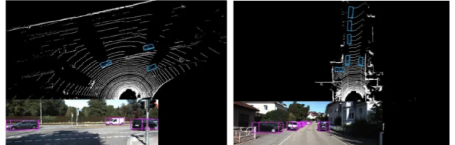
Left figure shows volumetric rendering. Right figure shows single 2D axial slice with handgun, bottle and artefacts indi-cated. From Flitton et al. (2015). . . 2 1.3 3D object detection in real world self-driving case. 3D Boxes
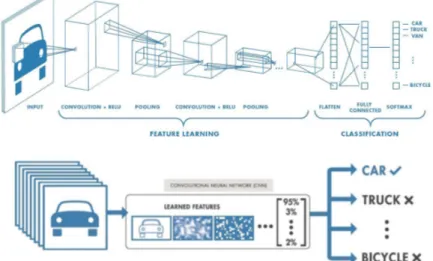
are projected to the bird’s eye view and the images. From Chen et al. (2017). . . 3 2.1 An CNN with eight different layers works on the task of
identifying a car. It learns features based on local group of pixels and combines the information together through layers to generate a set of probabilities. . . 7 2.2 Convolutional neural network break down: calculation with
a 3-by-3 kernel and three different color channels. . . 8 3.1 CNN representation. It is similar to Figure 2.1 except for
generalizing two-dimensional case to three-dimensional case. From Wu et al. (2014). . . 12 3.2 Example flowcharts show the overall procedure of VoxNet
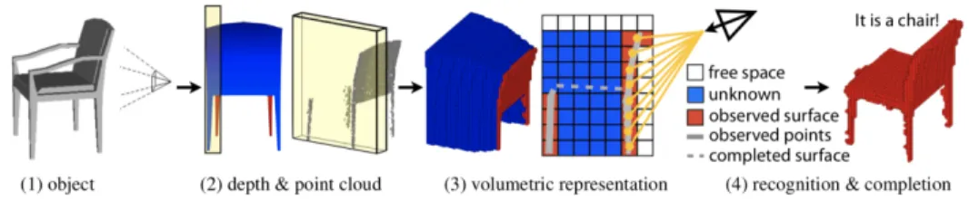
and Vote3D. . . 13 3.3 View-based 2.5D Object Recognition. (1) A depth map is taken
from a physical object. (2) The depth image is captured from the back of the chair. (3) The profile of the slice and different types of voxels. (4) The recognition and shape completion result, conditioned on the observed free space and surface. . 14
viii List of Figures
3.4 Each subdivision step halves the edge lengths, increases the number of faces by a factor of 4, and reduces the approximation error by a factor of about 1/4. From Botsch et al. (2010). . . . 16 3.5 Mesh pooling operates on irregular structures and adapts
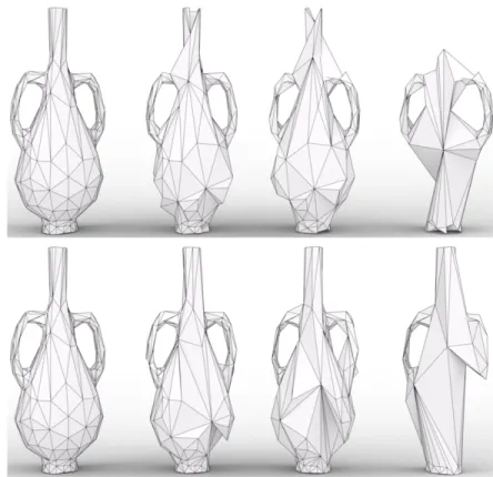
spatially to the task. Unlike geometric simplification, mesh pooling delegates which edges to collapse to the network. Top: MeshCNN trained to classify whether a vase has a handle, bottom: trained on whether there is a neck. From Hanocka et al. (2018). . . 17 3.6 Example of representation of a triangular mesh. The 1-ring
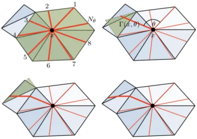
neighbors of e can be ordered as(a,b,c,d)or(c,d,a,b). This ambiguates the convolutional receptive field, hindering the formation of invariant features. . . 18 3.7 Constructed a local geodesic polar coordinates on a triangular
mesh. From Masci et al. (2015). . . 19 3.8 Determination of the formula for shading. This model is
abstracted into thex−y−zcoordinates while light comes from thezaxis. From Phong (1975). . . 21 3.9 Multi-view CNN for 3D shape recognition is illustrated here.
At test time a 3D shape is rendered from 12 different views to extract view based features. These are then pooled across views to obtain a compact shape descriptor. . . 22 3.10 PointNet CNN takes n points as input, applies input and
feature transformations, and then aggregates point features by max pooling. The output is classification scores for k classes. From Qi et al. (2016). . . 24 3.11 Diagrams show examples of max pooling layers. Left image is
a pictorial explanation in two-dimensional matrix case. Right image is a real life application on three dimensional vision data. 25 3.12 While critical points jointly determine the global shape feature
for a given shape, any point cloud that falls between the critical points set and the upper bound shape gives exactly the same feature. . . 28 3.13 Pipeline of generating Eigen-shape descriptor and
Fisher-shape descriptor. A collection of Heat Fisher-shape descriptors are used to train Principal Component Analysis (PCA) and Lin-ear Discriminant Analysis (LDA). The trained Eigen-shape descriptors are illustrated on the right and Fisher-shape de-scriptors are shown on the left. From Fang et al. (2015). . . . 31
List of Figures ix
3.14 The geometric feature DNN can extract features of various
parts from a single object. From Guo et al. (2015) . . . 32
3.15 Compiles a knowledge matrix requires calculation of geomet-ric features from each object and comparison between each pair of objects. Then a logical judgement process will be used to classify based on information in the knowledge matrix. From Ma et al. (2018). . . 32
4.1 Flowchart shows the logic of further explorations. . . 36
5.1 An intuitive understanding of alpha-shape in 2D case can be expressed by the circles as the metaphored ice-cream spoons. From Edelsbrunner and Mücke (1994). . . 40
5.2 Anα-exposed ball (left) doesn’t contain any other point while a nonα-exposed ball does (right). . . 41
5.3 Boundary of an alpha-shape . . . 42
5.4 Original 3D shape. This example will be used throughout the chapters for other illustration. . . 45
5.5 All 2D level sets of a 3D object (chair). . . 45
5.6 α-Shape with 4 differentαs: 0.01, 0.5, 1, 2. . . 46
5.7 Findα-shape of all level sets. . . 46
5.8 3Dα-shape result. . . 47
6.1 Logarithmic curve example . . . 50
6.2 Example of curvature for various curves. . . 51
6.3 Findα-shape of all level sets. . . 52
6.4 Different cubic splines result . . . 53
6.5 The principal curvatures at a point on a surface. . . 54
6.6 The Gauss map sends a point on the surface to the outward pointing unit normal vector, a point onS2. . . 55
7.1 Findα-shape of all level sets. . . 58
7.2 Correspondence between the geometric features and the original object. . . 59
8.1 ModelNet10 data example . . . 64
8.2 ModelNet10 model size . . . 64
8.3 Re-visit the system flowchart: adding geometric features to CNN . . . 65 8.4 Re-visit the system flowchart: using geometric without CNN 65
List of Tables
Acknowledgments
I would like to express my deepest appreciation to Professor Weiqing Gu for all her instructions and help which is crucial for my thesis works, as well as all her encouragement and patience. Without her guidance and persistent help this thesis wouldn’t be completed.
I’d like to extend my gratitude to Professor Nicholas Pippenger who agrees to be my second reader, especially for the useful comments on my thesis draft.
In addition, I’d like to thank Professor Jon Jacobsen for his encouragement in the middle of my thesis when I was feeling extremely unsure about my work.
Special thanks to all the professors, staff and my friends from Harvey Mudd College Department of Mathematics whose assistance was a milestone in the completion of this thesis.
Chapter 1
Introduction to 3D Object
Classification
The so-called 3D object classification task is easy to interpret right from its name, even without any math or computer science background. To do 3D object classification simply means that given a certain object, represented in 3D form with either points, surfaces or other information specified, we would like to decide what this object is. For example, given a set of points comprising the skeleton of a thin rectangular board with four thin and long legs under it, we would argue that it’s possibly a table, but not a television. If there is another rectangular shape put vertically on the top of the board, it’s likely a chair. (See Figure 1.1 for example.)
Figure 1.1 Point clouds of a chair and a table, which are likely the object of what 3D object classification will study. Adopted from the ShapeNet Core55 dataset.
2 Introduction to 3D Object Classification
Figure 1.2 Example baggage-CT scan containing handgun and bottle. Left figure shows volumetric rendering. Right figure shows single 2D axial slice with handgun, bottle and artefacts indicated. From Flitton et al. (2015).
Apparently, the task of 3D object classification is not hard for human eyes. In our daily life, every moments our eyes take in information about the surrounding world and decide what the objects are. We could never possibly confuse a normal chair with a table. This is definitely partly because of the plenty of details we can see, including colors, texture, shape, etc. But as in Figure 1.1, even with very basic point clouds, human eyes can decide what the object is without any difficulties. This is because we can detect the shape, orgeometricinformation from the objects.
However, there are also lots of cases where we need computers, instead of human eyes, to classify and identify the objects. Especially with the recent availability of inexpensive 2.5D depth sensors (e.g. Microsoft Kinect, Intel RealSense, Google Project Tango, and Apple Prime-Sense). For example, in security check of airports of train stations, a single camera view will provide scan information of a baggage and we need to identify if there’s any dangerous objects in the baggage. Flitton et al. (2015) investigates the performance of a Bag of (Visual) Words (BoW) object classification model as an approach for automated threat object detection within 3D Computed Tomography (CT) imagery from a baggage security context (Figure 1.2). Zheng et al. (2009) shows the possibility of applying this technology to medical areas with their projects, which use Marginal Space Learning (MSL) to automatically detect 3D anatomical structures in many medical imaging modalities. Chen et al. (2017) proposes Multi-View 3D networks (MV3D), a sensory-fusion framework that takes both LIDAR point cloud and RGB images as input and predicts oriented 3D bounding boxes used in self-driving vehicles (1.3).
A brief review of existing 3D object classification technologies show that deep learning and especially deep neural network plays a significant role in recent 3D object classification algorithms. Dating back to previous years,
3
Figure 1.3 3D object detection in real world self-driving case. 3D Boxes are projected to the bird’s eye view and the images. From Chen et al. (2017).
deep learning had long shown great potentiality and application in 2D object classification, detection and identification tasks, especially with the help of the new larger datasets include LabelMe by Russell et al. (2008), which consists of hundreds of thousands of fully-segmented images, and ImageNet by Li et al. (2010), which consists of over 15 million labeled high-resolution images in over 22,000 categories. Researchers include Krizhevsky et al. (2017) and Ciresan et al. (2012) explored 2D image classification and achieved very competitive accuracy with deep learning approaches.
While more and more high-quality data sets become available and the computation ability of devices significantly increases, the emphasis in object classification field in computer vision has gradually moved from 2D classification (or image classification) to directly working with 3D point set data that efficiently, directly and accurately models real life problems.
Considering 3D object classification as an interesting, worth studying and developing area, this thesis aims to review, study and compare some of the notable existing algorithms with high performance. Starting from next chapter, the theories of algorithms including the so-called Convolutional Neural Network (CNN) will be introduced. Future chapters after those will introduce how geometric ideas will be compared and combined into existing technologies.
Chapter 2
Introduction to Convolutional
Neural Network
Up to now, the most popular method that produces most of the state-of-the-art algorithms with good performance is classification with Artificial Neural Networks (ANN) models, especially Convolutional Neural Notworks (CNNs). These systems are able to learn how to perform tasks by considering examples, generally instead of being explicitly programmed with domain-specific rules. This is not surprising because CNN is already proved to be a fruitful approach in 2-dimensional cases. This chapter will begin with a brief introduction to the mathematical background of artificial neural network, and then focus on discussing CNN.
Definition 2.1. Afeedforward neural network, aka multi-layer perceptron (MLP), is a series of logistic regression models stacked on top of each other, with the final layer being either another logistic regression or a linear regression model, depending on whether we are solving a classification or regression problem. (Murphy (2012))
Suppose a MLP used to solve regression problem has two layers, then it can be mathematically expressed as
p(y|x,θ)N y|wTz(x), σ2 z(x) g(Vx) g vT
1x
, . . . ,g vTHx
wheregis a non-linear activation or transfer function (commonly the logistic function),z(x)φ(x,V)is called the hidden layer (a deterministic function of the input),His the number of hidden units,Vis the weight matrix from
6 Introduction to Convolutional Neural Network
the inputs to the hidden nodes, andwis the weight vector from the hidden nodes to the output.
Theorem 2.1. An MLP is a universal approximator, meaning it can model any suitably smooth function, given enough hidden units, to any desired level of accuracy.
Hornik (1991) proved Theorem 2.1 twenty years ago, making a solid stepping stone for other further usage of MLP to various computer-related tasks. The underlying meaning here is that as long as the computing power allows a certain number of hidden units, any smooth function underlying the regression or classification tasks should be able to be approximated by deep neural network.
The purpose of the hidden units is to learn non-linear combinations of the original inputs; this is calledfeature extractionor feature construction. These hidden features are then passed as input to the final generalized linear model.
This approach is particularly useful for problems where the original input features are not individually informative. For example, each pixel in an image is not very informative; it is the combination of pixels that tells us what objects are present. Conversely, for a task such as document classification using a bag of words representation, each feature (word count) is informative on its own, so extracting "higher order" features is less important (Murphy (2012)).
The so-called Convolutional Neural Network (CNN) is a special and widely-used type of neural network. The name "convolutional neural network" indicates that the network employs a mathematical operation called
convolution. Convolutional layers have analogy in human neuroscience, which is actually the origin and conceptual background of all neural network models. Then convolve the input and pass its result to the next layer, which is similar to the response of a neuron in the visual cortex to a specific stimulus. Each convolutional neuron processes data only for its receptive field.
For a more mathematically rigorous definition, convolution is a special-ized kind of linear operation. Convolutional networks are by definition neural networks that replace general matrix multiplication with convolution in at least one of the layers.
Definition 2.2. Convolutionis the process of taking a small matrix of real numbers (called kernel or filter), passing it over our image and transforming
7
the image based on the filter values.
G[m,n](f∗h)[m,n]Õ j
Õ
k
h[j,k]f[m−j,n−k]
where f is the input data andhis the kernel.
With the Definition of convolution, (Definition 2.2), we can specify the following definition of Convolutional Neural Network.
Definition 2.3. AConvolutional Neural Networkis an MLP in which the hidden units have local receptive fields, and in which the weights are tied or shared across the data (usually image), in order to reduce the number of parameters. (Murphy (2012))
Figure 2.1 An CNN with eight different layers works on the task of identify-ing a car. It learns features based on local group of pixels and combines the information together through layers to generate a set of probabilities.
A convolutional neural network can assign importance (learnable weights and biases) to various aspects or parts in the input data and be able to differentiate one from the other. Intuitively, the effect of such spatial parameter tying is that any useful features that are "discovered" in some portion of the data can be re-used everywhere else without having to be independently learned. (Murphy (2012)) The resulting network then exhibits
8 Introduction to Convolutional Neural Network
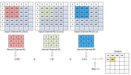
Figure 2.2 Convolutional neural network break down: calculation with a 3-by-3 kernel and three different color channels.
translation invariance, meaning it can classify patterns no matter where they occur inside the input data.
Figure 2.1 shows how a convolutional neural network works on a 2D image case. In order to identify a car, each layer of the neural network picks some details of the original image and uses a specially designed filter to catch important information. Finally the image is summarized into a list of data representing what the filter "think" is important in the image. Not surprisingly, just as in this case, convoluitonal neural networks are mostly applied to visual pattern recognition.
Figure 2.2 provides a mathematical breakdown of what a CNN does. In this case, it has a 3-by-3 filter that goes through the whole matrix, multiply with the sub-matrices, and produces results in a compressed form for each color channel of an image. Different filters could be designed for specific tasks, like edge detection.
Previous studies and those illustrations above shows clearly how con-volutional network is promising in the area of 2D image processing. When problem comes to three-dimensional, however, things become much more complex. The data form of 2D images are simple in that all images can be represented with a uniform representation ofpixels. In Figure 2.2, we have three matrices representing the values of three color channel on each single location of an image. However, this is not the only intuitive representation for
9
3D data, especially sparse data. Consider a chair object with no background, instead of pixel values, it might be more intuitive to view it as a cloud of points with surfaces covering the points. Some object might be hard to view inside structures, and some objects can only be viewed from several angle as 2D rendering images. All these problems remind us that although it’s a great insight to generalize CNN to 3D case, we need to solve the problem of choosing the rightrepresentationbeforehand. The next few chapters will discuss several widely used representations, including their strength and weakness.
Chapter 3
Previous Works
3.1
Volumetric Convolutional Neural Network
3.1.1 A Single Naive Representation: VoxelAs a beginning, we will start from the most intuitive generalization from 2D image to 3D object representation. When dealing with two-dimensional image data, we in fact consider it as a huge matrix of tuples, where each element in a single tuple, is a pixel indicating the color or transparency of that certain location on the graph. It’s natural, then, to extend this notion to a 3D grid with unit cube calledvoxel.
Definition 3.1. A voxel represents a value on a regular grid in three-dimensional space.
The so-called voxel representation is the most widely used, traditional and popular approach. Wu et al. (2014) was the first research group introducing this groundbreaking approach which represents a geometric 3D shape as a probabilistic distribution of binary variables on a 3D voxel grid, and they applied it into 3D classification. Each 3D mesh is represented as a binary tensor: 1 indicates the voxel is inside the mesh surface, and 0 indicates the voxel is outside the mesh (i.e., it is empty space).
Wu et al. (2014) used Convolutional Deep Belief Network (CDBN), which is a powerful class of probabilistic models often used to model the joint probabilistic distribution over pixels and labels in 2D images. This is directly adopted from 2D image cases, again showing why this voxel representation is natural and intuitive.
12 Previous Works
1. A volumetric grid representing our estimate of spatial occupancy. 2. A 3D CNN that predicts a class label directly from the occupancy grid.
Theorem 3.1. The energy,Eof a convolutional layer can be computed as:
E(v,h)−Õ f Õ j hjf Wf ∗v j+c fhf j −Õ l blvl
wherevl denotes each visible unit,hjf denotes each hidden unit in a feature channel f, andWf denotes the convolutional filter.
Figure 3.1 CNN representation. It is similar to Figure 2.1 except for generalizing two-dimensional case to three-dimensional case. From Wu et al. (2014).
Theorem 3.1 shows how the energy of a convolutional layer is calculated in their CNN model. It’s a traditional model with visible units, hidden units, and a convolutional layer (a more complex version of the 3-by-3 matrix filter shown in Figure 2.2). Although this is not a very specifically designed method, it’s extraordinary at its time because it’s actually the first
Volumetric Convolutional Neural Network 13
CNN-based 3D object classification algorithm with good performance, and provides motivation for a great number of following researchers.
After training the CNN, the model learns the joint distributionp(x,y)of voxel dataxand object category labely ∈ {1,· · · ,K}.
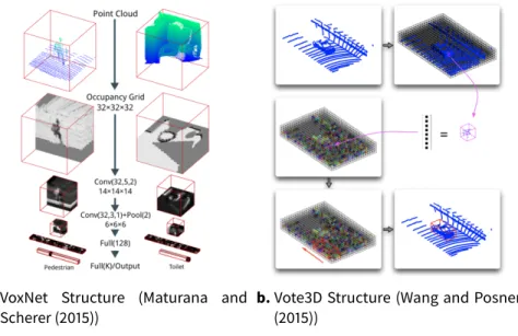
After them, other researchers improved the volumetric representation by adding details and fine-tuning the neural network for different datasets. Maturana and Scherer (2015) proposed VoxNet that integrated a volumetric occupancy grid representation with a supervised 3D CNN, which signifi-cantly improved the performance. Shi et al. (2015) converted each 3D shape into a panoramic view, namely a cylinder projection around its principle axis, and thus developing a robust representation called DeepPano. Zhao et al. (2019) considered the normal vectors after voxelized the input. He et al. (2015) presented a residual learning framework to ease the training of networks that are substantially deeper than those used previously.
a.VoxNet Structure (Maturana and Scherer (2015))
b.Vote3D Structure (Wang and Posner (2015))
Figure 3.2 Example flowcharts show the overall procedure of VoxNet and Vote3D.
In general, the volumetric CNN approach abstracts the information stored in 3D point cloud to free, occupied and unknown voxels, thus turning irregular data into regular representations. This distinction among three types provides an extremely rich information in representation, while can be stored in easy and structured data form. However, a noticeable weakness of this approach is that it requires lots of memory and computation, which
14 Previous Works
Figure 3.3 View-based 2.5D Object Recognition. (1) A depth map is taken from a physical object. (2) The depth image is captured from the back of the chair. (3) The profile of the slice and different types of voxels. (4) The recognition and shape completion result, conditioned on the observed free space and surface.
greatly restricts the amount of data it could take in as training set.
Additionally, voxelized approach ignores the extent of sparsity in 3D data representation: even though a large majority of the space are not occupied at all, the "empty" information will be marked with equal significance as the "occupied" information. Wang and Posner (2015) illustrates an approach that differs in that its nature comes from the sliding window algorithm widely used in 2D image processing. Wang and Posner generalizes this idea to 3D cases, replacing a sliding square to a sliding window. Compared with the most generic voxel-CNN, this idea specifies in dealing with sparsity in the input 3D point cloud.
3.1.2 Play with 2.5D Data
Note that up to the CNN step, only full completed data set is used to train the model and make predictions. However, as Wu et al. (2014) mentioned, it’s also possible to recover full 3D shapes from view-based 2.5D depth maps. Imagine the application with Microsoft Kinetic or other depth detection hardware: in Figure 3.3 when you have a depth map viewed from only one direction, only very limited knowledge is known about the 3D object. But the volumetric ShapeNet is able to construct a probabilistic model on the grids. That is, it will generate a probability for each voxel to be either free, occupied or unknown. This probability distribution then guides us to complete the full model based on assumptions. This shape completion functionality suggests that not the full information in dataset is necessary for generating a successful classification. Then the natural question arises: what points are necessary or important for generating a good classification? This topic will be explored again in further chapters.
Surface Polygon Mesh 15
3.2
Surface Polygon Mesh
3.2.1 Introduce MeshWhile the locations of points are one good representation and descriptor of 3D shape, another feature marks how 3D object is in nature different from 2D images: it has the so-called surface information that cannot be easily captured by voxelized data or point cloud data. This leads to another popular representation, which is called mesh.
Definition 3.2. The polygonal mesh representation, or mesh, for short, approximates surfaces via a set of 2D polygons in 3D space. (Botsch et al. (2010))
The mesh provides an efficient, non-uniform representation of the shape. Only a small number of polygons are required to capture large, simple, surfaces. On the other hand, representation flexibility supports a higher resolution where needed, allowing a faithful reconstruction, or portrayal, of salient shape features that are often geometrically intricate. (Hanocka et al. (2018))
The most basic and commonly used mesh is the so-calledtriangular mesh. It’s widely used in 3D object classification problem by representing the object with surface mesh information and build descriptors on that.
Definition 3.3. A triangle meshMconsists of a geometric and a topolog-ical component, where the latter can be represented by a graph structure (simplicial complex)with a set of vertices
V {v1, . . . ,vV} and a set of triangular faces connecting them
F f1, . . . , fF , fi ∈ V × V × V (Botsch et al. (2010))
The geometric embedding of a triangle mesh intoR3 is specified by associating a 3D positionpi to each vertexvi ∈ V :
P {p1, . . . ,pV}, pi :p(vi)© « x(vi) y(vi) z(vi) ª ® ¬ ∈ R3
16 Previous Works
Figure 3.4 Each subdivision step halves the edge lengths, increases the num-ber of faces by a factor of 4, and reduces the approximation error by a factor of about 1/4. From Botsch et al. (2010).
such that each face f ∈ F actually corresponds to a triangle in 3-space specified by its three vertex positions. Notice that even if the geometric embedding is defined by assigning 3D positions to the discrete vertices, the resulting polygonal surface is still a continuous surface consisting of triangular pieces with linear parameterization functions. Figure 3.4 shows and example of triangular mesh with different sizes.
Another significant characteristic of the mesh is its native provision of connectivity information. This forms a comprehensive representation of the underlying surface. Compared with the PointNet approach discussed in further chapters, mesh representation perfectly deals with the problem of connectivity and surface representation. The examplar work of Masci et al. (2015) introduced deep learning of local features on meshes and showed how to use these learned features for correspondence and retrieval. Haim et al. (2018) used toric topology to define the convolutions on the shape graph. Fouinat et al. (2018) defined a new convolutional layer that allows propagating geodesic information throughout the layers of the network. 3.2.2 Mesh CNN: Theory and Insight
As one of the pioneer work and currently one of the best performance system, Hanocka et al. (2018)’s system proposed a convolution on the edges of a mesh and also a learned mesh pooling operation that adapts to the task at hand, further expanding the research on meshes and significantly increased the performance. Note that in Figure 3.5, the most traditional non-uniform triangular mesh was used: large flat regions use a small number of large triangles, while detailed regions used a larger number of triangles.
The input edge feature for each edge is a five-dimensional vector including the dihedral angle, two inner angles and two edge-length ratios for each
Surface Polygon Mesh 17
Figure 3.5 Mesh pooling operates on irregular structures and adapts spatially to the task. Unlike geometric simplification, mesh pooling delegates which edges to collapse to the network. Top: MeshCNN trained to classify whether a vase has a handle, bottom: trained on whether there is a neck. From Hanocka et al. (2018).
face. The edge ratio is between the length of the edge and the perpendicular (dotted) line in Figure 3.6 for each adjacent face. The researchers sorted each of the two face-based features (inner angles and edge-length ratios), thereby resolving the ordering ambiguity and guaranteeing invariance. Observe that these features are all relative, making them invariant to translation, rotation and uniform scale. (Hanocka et al. (2018).)
However, compared with the geometric feature representation, the mesh representation is not as natural and intuitive if considering how human eyes actually recognize objects: most of the objects have smooth shape, like the vase shown in Figure 3.5 in real life won’t be recognized as composing
18 Previous Works
Figure 3.6 Example of representation of a triangular mesh. The 1-ring neigh-bors of e can be ordered as(a,b,c,d)or(c,d,a,b). This ambiguates the
con-volutional receptive field, hindering the formation of invariant features.
of small polygons. The success of mesh representation again urges us to explore if there’s some more natural way to enhance it by mimicing how human eyes approach the identification task.
3.2.3 Local Polar Coordinate
Before introducing a more advanced technique also based on the idea of mesh, let’s define the concept of manifold and Riemannian Manifolds, which will also be used in further chapters.
Definition 3.4. A manifold is a topological space that locally resembles Euclidean space near each point. More precisely, each point of an n -dimensional manifold has a neighborhood that is homeomorphic to the Euclidean space of dimensionn.
The rich theory of vector spaces endowed with a Euclidean inner product can, to a great extent, be lifted to various bundles associated with a manifold. The notion of local (and global) frame plays an important technical role.
Definition 3.5. Let M be an n-dimensional smooth manifold. For any open subset, U ⊆ M, an n-tuple of vector fields, (X1, . . . ,Xn), overU is called a frame overUiff X1(p), . . . ,Xn(p)is a basis of the tangent space, TpM, for every p ∈ U. If U M, then the Xi are global sections and (X1, . . . ,Xn) is called a frame (ofM)
Surface Polygon Mesh 19
Now we could define a Riemannian manifold.
Definition 3.6. Given a smoothn-dimensional manifold,M, a Riemannian metric on M is a family, h−,−ip
p∈M,of inner products on each tangent space,TpM,such thath−,−ip depends smoothly onpwhich means that for every chart,ϕα :Uα→Rn,for every frame,(X1, . . . ,Xn),onUα,the maps
p 7→Xi(p),Xj(p)
p, p ∈Uα, 1≤i,j≤ n
are smooth. A smooth manifold,M,with a Riemannian metric is called a Riemannian manifold.
Figure 3.7 Constructed a local geodesic polar coordinates on a triangular mesh. From Masci et al. (2015).
Geodesic Convolutional Neural Networks can be considered as another kind of geometric feature recognition based on Riemannian Manifolds. GCNN is a natural generalization of the convolutional networks (CNN) paradigm to non-Euclidean manifolds. Researchers’ construction is based on a local geodesic system of polar coordinates to extract "patches“, which are then passed through a cascade of filters and linear and non-linear operators.
Masci et al. (2015) model a 3D shape as a connected smooth compact two-dimensional manifold (surface)X,possibly with a boundary∂X.Locally around each pointxthe manifold is homeomorphic to a two-dimensional
20 Previous Works
Euclidean space referred to as the tangent plane and denoted byTxX.A Riemannian metric is an inner product h·,·iT
xX : TxX×TxX → Ron the tangent space depending smoothly onx.
Basically, how GCNN works is by building a local polar coordinate system to represent the information in a 3D object. Broadly speaking, a local feature descriptor assigns to each point on the shape a vector in some multi-dimensional descriptor space representing the local structure of the shape around that point. A global descriptor describes the whole shape, which is harder to establish and not used in this algorithm.
3.3
Multi-View Convolutional Neural Network
While representations like voxel grid or polygon mesh are considered descriptors operating on their native 3D formats, another possible direction is to represent data in a view-based term. In another word, is it possible to recognize 3D shapes from a collection of their rendered views on 2D images? Answering this question, Su et al. (2015) provides a different approach in lots of CNN attempts by tracking the 3D problem back to 2D. They tried to render 3D point cloud or shapes into 2D images and then applied 2D CNN to classify them. Even the first step of classifying only with a single rendered image shows better performance than some state-of-the-art 3D object recognition approaches. After that, they designed a special algorithm also by convolutional neural network to combine several 2D classification result of a single object to get an overall shape descriptor that leads to even more accurate prediction performance.
3.3.1 Build Rendered 3D Models
3D models in online databases are typically stored as polygon meshes, which are collections of points connected with edges forming faces. To generate rendered views of polygon meshes, Su et al. (2015) used the Phong reflection model (Phong (1975)) which basically consists of two parts:
1. Render the mesh polygons under a perspective projection. This type of representation has the advantage that it avoids the problem posed by mathematically curved surface approaches, of solving higher order equations.
2. Determine the pixel color by interpolating the reflected intensity of the polygon vertices. Taking into consideration that the light received
Multi-View Convolutional Neural Network 21
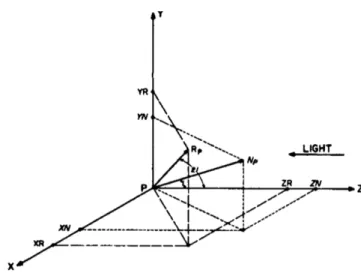
Figure 3.8 Determination of the formula for shading. This model is abstracted into thex−y−zcoordinates while light comes from thezaxis. From Phong (1975).
by the eye is provided one part by the diffuse reflection and one part by the specular reflection of the incident light, the shading at pointP on an object can be computed as:
Sp Cp[cos(i)(1−d)+d]+W(i)[cos(s)]n
where Cp is the reflection coefficient of the object at point P for a certain wavelength. iis the incident angle. d is the environmental diffuse reflection coefficient. Wi is a function which gives the ratio of the specular reflected light and the incident light as a function of the incident anglei. s is the angle between the direction of the reflected light and the line of sight. nis a power which models the specular reflected light for each material.
After building the 3D shape, the researchers actually setup viewpoints (so-called virtual cameras) to create a multi-view shape representation. In Figure 3.9, it shows how twelve cameras are set up around the object chair and twelve images will be produced and classified by each camera.
3.3.2 Detailed CNN Design for Aggregation
In classification and retrieval test, the most crucial part is how to aggregate the results from all those different rendered cameras. The following theorem
22 Previous Works
Figure 3.9 Multi-view CNN for 3D shape recognition is illustrated here. At test time a 3D shape is rendered from 12 different views to extract view based features. These are then pooled across views to obtain a compact shape descriptor.
provides a metric to calculate the distance between two 3D objects by computing allnx×nypairwise distances between images. Simply averaging or concatenating the image descriptors leads to inferior performance.
Theorem 3.2. Distance between two 3D shapes are defined as
d(x,y) Í jmini xi −yj 2 2ny + Í iminj xi −yj 2 2nx
Herex,yrepresent the two 3D objects. xi,yj represents the view from each camera, withi,jgoing from 1 to the number of cameras. In a word, we take the sum of the minimum of distance between views, which help us rectify the possible rotation of the objects, then take the average to decide the estimated distance between objects.
Result shows that 2D information can be highly informative to 3D struc-tures. This method significantly increases spatial resolution (although with less explicit depth information) compared to CNNs taking 3D information as input. It can also take advantage of the much more mature and abun-dant pre-trained models and data sets of 2D object classification, including LabelMe by Russell et al. (2008) and ImageNet by Li et al. (2010) discussed before.
3.3.3 Advanced Related Works
Yan et al. (2016) discussed Perspective Transformer Nets that formulated the learning process as an interaction between 3D and 2D representations and proposed an encoder-decoder network with a novel projection loss
PointNet: Direct Point Cloud Representation 23
defined by the perspective transformation. The projection loss enabled the unsupervised learning using 2D observation without explicit 3D supervision. Gao et al. (2018) explored pairwise multiview information and introduced a novel pairwise Multi-View Convolutional Neural Network for 3D Object Recognition (PMV-CNN for short), where automatic feature extraction and object recognition were put into a unify CNN architecture.
Large scale experiments demonstrate that the pairwise architecture is very useful when the number of labeled training samples is very small. Recent researches on multi-view representation basically focused on two directions: multi-view matching and label propagation. An exemplar research in the former area is Wang et al. (2012) which used manifold to manifold distance. The later one is generally related with graph propagation (Gao et al. (2012)).
This approach is intuitive and also widely used at the beginning because the huge number of developed, available dataset and technology for 2D image classification. Evolving from 2D to 3D in this sense is probably the most intuitive approach for experienced researchers. However, the propagation algorithm that builds the bridge from 2D to 3D is not robust enough. For example, Theorem 3.2 used to calculate the distance between 2 objects is still in a primary form. Although it’s designed to handle rotation and different angle, it’s not elaborated enough to handle all subtle cases.
Moreover, the greatest problem for this approach is still that the camera photo could only take care of outside features. For example, if there’s a hole inside the object or some subtle features that is blocked from direct sight but can be reflected by 3D point cloud, the camera couldn’t take care of that. Especially if an object is not convex, several camera views will produce significant torsion.
3.4
PointNet: Direct Point Cloud Representation
3.4.1 Point Cloud Representation: Opportunity and Challenges The most basic and naive form of 3D object representation should be simply a cloud of 3D points, embedding in thex−y−zcoordinate, each represented as a tuple of(x,y,z). Obviously, it’s not possible to take all points from a single object. So, depending on the density and location of these points, the level of difficulty varies. Besides the problem of point density, the 3D point cloud representation has the following few features (Qi et al. (2016)):24 Previous Works
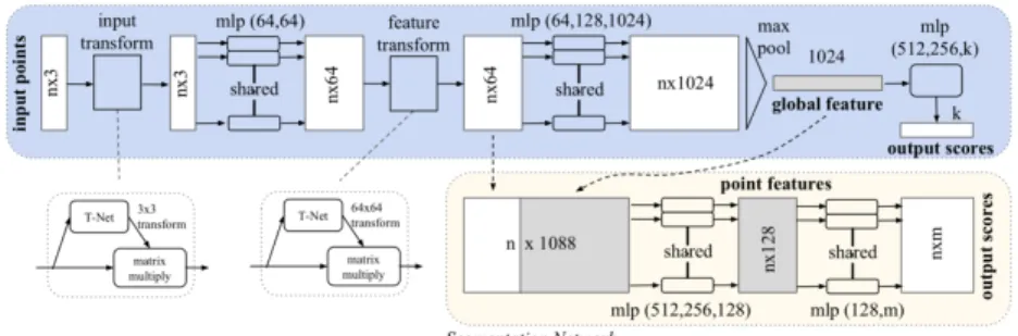
Figure 3.10 PointNet CNN takesnpoints as input, applies input and feature transformations, and then aggregates point features by max pooling. The output is classification scores forkclasses. From Qi et al. (2016).
1. Unordered. Unlike volumetric representation, a set of points is not assigned in a special order. A network that consumes N 3D point sets needs to be invariant toN! permutations of the input set in data feeding order.
2. Interaction among points. The points are from a space with a distance metric. It means that points are not isolated, and neighboring points form a meaningful subset. Therefore, the model needs to be able to capture local structures from nearby points, and the combinatorial interactions among local structures.
3. Invariance under transformations. As a geometric object, the learned representation of the point set should be invariant to certain transforma-tions. For example, rotating and translating points all together should not modify the global point cloud category nor the segmentation of the points.
Based on this idea, Qi et al. (2016) presented a modern neural network approach that instead of using CNNs on voxels, takes the raw 3D point cloud data as input. That is, each point is represented by just its three coordinates (x,y,z). Because of the three features mentioned before, it takes special care to design a specific CNN model that satisfies the features of point cloud. Qi et al. (2016)’s algorithm learned optimization function that select interesting or informative points. Then the fully connected layers aggregated these learnt optimal values into the global descriptor and did classification or segmentation. The whole architecture is shown in the block diagram in Figure 3.10.
PointNet: Direct Point Cloud Representation 25
Figure 3.11 Diagrams show examples of max pooling layers. Left image is a pictorial explanation in two-dimensional matrix case. Right image is a real life application on three dimensional vision data.
3.4.2 Max Pooling Layer for Special Features
What’s important and unique in this neural network structure are the three specific features designed to accommodate the special properties of point cloud, especially using symmetric function and max pooling layer to make the model invariant to input permutation.
Definition 3.7. Max pooling is a sample-based discretization process. The objective is to down-sample an input representation (image, hidden-layer output matrix, etc.), reducing its dimensionality and allowing for assump-tions to be made about features contained in the sub-regions binned. (Anand J. Kulkarni and Suresh Chandra Satapathy (2020))
In another word, max pooling layer does nothing more than dividing the data into small sections, and take the maximum point of each section to represent the whole bundle. This is used to reduce the size of data and can easily catch the prominent features. Figure 3.11 shows two examples on calculating max pooling layer by hand. In the left image, for example, we want to take each small square of 2 by 2 dimension and use the single maximum number to represent it, resulting in a matrix that is four times smaller.
We value the max pooling function for the sense of symmetric it shows in nature. In order to make the model invariant to input permutation, it’s convenient to use a simple symmetric function to aggregate the information from each point. The high level idea behindPointNetis to approximate a
26 Previous Works
general function defined on a point set by applying a symmetric function on transformed elements in the set, illustrated by Theorem 3.3 below.
Theorem 3.3. f ({x1, . . . ,xn}) ≈ g(h(x1), . . . ,h(xn)) where f : 2RN →R,h:RN →RKand g:RK× · · · ×RK | {z } n →Ris a symmetric function.
By Theorem 3.3, the idea of PointNet is to approximate a general function defined on a point set by applying a symmetric function on transformed elements in the set. Empirically, this module is very simple: it approximates hby a multi-layer perceptron network and g by a composition of a single variable function and a max pooling function. Through a collection ofh,we can learn a number of f0s to capture different properties of the set.
Theorem 2.1 already shows that MLP can model any suitably smooth function, given enough hidden units, to any desired level of accuracy. In this case where we add the max pooling layers, it’s also required to show the universal approximation ability of the neural network to continuous set functions.
3.4.3 Arbitrarily Approximate and Critical Point
For a more mathematical rigorous explanation of the theory behind, let’s start with a few background definition.
Definition 3.8. LetX and Ybe two non-empty subsets of a metric space (M,d).We define their Hausdorff distancedH(X,Y)by
dH(X,Y)max ( sup x∈X∈Y d(x,y), sup y∈Y∈X d(x,y) )
where sup represents the supremum and infthe infimum. Equivalently dH(X,Y)inf{ε ≥0;X ⊆YεandY ⊆Xε}
where
Xε: Ø x∈X
{z ∈ M;d(z,x) ≤ ε}
that is, the set of all points withinεof the setX (sometimes called theε -fattening ofXor a generalized ball of radiusεaroundX).
PointNet: Direct Point Cloud Representation 27
Formally, letX{S:S ⊆ [0,1]m and|S| n}, f :X →Ris a continu-ous set function onXw.r.t to Hausdorff distancedH(·,·),i.e.,∀ >0,∃δ >0, for anyS,S0∈ XifdH(S,S0)< δ,
thenf(S) − f(S0)
< .Then Theorem 3.4 below says that f can be arbitrarily approximated by our network given enough neurons at the max pooling layer, i.e.,Kis sufficiently large.
Theorem 3.4. (Qi et al. (2016)) Suppose f : X → R is a continuous set
function w.r.t Hausdorff distancedH(·,·). ∀ >0,∃acontinuous functionhand asymmetric function g(x1, . . . ,xn)γ◦MAX,such that for anyS∈ X
f(S) −γ MAXxi∈S{h(xi)} <
wherex1, . . . ,xnis the full list of elements inSordered arbitrarily,γis a continuous
function, and MAX is a vector max operator that takes n vectors as input and returns a new vector of the element-wise maximum.
With this in mind, we can go back to the beginning of the chapter, where we raise the question about density of points for describing a 3D object. In fact, Theorem 3.5 below argues that for any 3D point cloud object, only part of the points are required to successfully identify the object.
Theorem 3.5. (Qi et al. (2016)) DefineuMAX xi∈S
{h(xi)}to be the sub-network
of f which maps a point set in[0,1]m to aK-dimensional vector.
Suppose u :X →RKsuch thatuMAX xi∈S
{h(xi)}and f γ◦u.Then
1. ∀S,∃CS,NS ⊆ X, f(T) f(S)ifCS⊆T ⊆ NS
2. |CS| ≤K
To prove this theorem, notice that obviously,∀S∈ X, f(S)is determined by u (S). So we only need to prove that ∀S,∃CS,NS ⊆ X, f(T) f(S)if CS ⊆T ⊆ NSFor the jth dimension as the output ofu,there exists at least one xj ∈ X such that hj xj uj, where hj is the jth dimension of the output vector fromh.TakeCSas the union of allxj for j1, . . . ,K.Then, CSsatisfies the above condition.
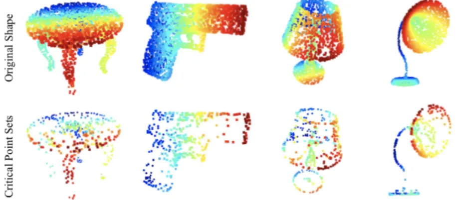
(1) says that f(S)is unchanged up to the input corruption if all points in CSare preserved; it is also unchanged with extra noise points up toNS. (2) says thatCSonly contains a bounded number of points, determined byKin (1). In other words, f(S)is in fact totally determined by a finite subsetCS ⊆S of less or equal toKelements. We therefore callCSthe critical point set of SandKthe bottleneck dimension of f.Note that this set of critical points
28 Previous Works
Figure 3.12 While critical points jointly determine the global shape feature for a given shape, any point cloud that falls between the critical points set and the upper bound shape gives exactly the same feature.
are different from the so-called critical points in the definition of differential geometry.
Compared with the voxelized approaches, this representation is much more direct and takes less voluminous input. Also it doesn’t require the input to be quantized, and thus saving lots of important information. But the most severe problem of it is that while considering point cloud information, it selectively ignores surface information, local features and connectivity status.
Further work on PointNet-liked CNNs generally aimed to improve its ability to recognize local feature and topological structure. Qi et al. (2017) then further improved the PointNet model’s performance by introducing a hierarchical neural network that applies PointNet recursively on a nested partitioning of the input point set. By exploiting metric space distances, this network is able to learn local features with increasing contextual scales. Shi et al. (2018) developed PointRCNN based upon the original PointNet model, which is a bottom-to-up 3D proposal generation method directly generates robust 3D proposals from point clouds, which is both efficient and quantization free. Guerrero et al. (2017), similarly, attempted to improve PointNet’s performance by extracting local features directly from point cloud.
Geometric Feature Extraction 29
3.5
Geometric Feature Extraction
Traditional methods explored and included some non-neural network ap-proaches to this problem, including SVM, Bayes model, propagational graph, and feature extraction.
3.5.1 Shape Descriptor
Fang et al. (2015) firstly converted the 3D data into a vector, by extracting traditional shape features and then use a fully connected net to classify the shape. To explore deeper into their work, we need to first define what is a shape signature and what is a shape descriptor, the representation they used to describe a 3D object.
Definition 3.9. 3D shape signatures and descriptors are succinct and compact representations of 3D object that capture the geometric essence of a 3D object. Shape signature is referred to as a local description for a point on a 3D surface and shape descriptor is referred to as a global description for the entire shape. (Fang et al. (2015))
Hand-crafted shape descriptors are sometimes not robust enough in order to solve the problem of structural variations present in 3D models. Discriminative feature learning from large datasets provides an alternative way to construct deformation-invariant features. This method has been widely used in computer vision and image processing. Specifically, there are three types of traditional shape descriptors with relatively good performance introduced in the sections below. (Fang et al. (2015)).
Heat shape descriptor (HeatSD)
The 3D model is represented as a graphG(V,E,W),whereVis the set of vertices,Eis the set of edges, andW represents the weight values for the edges. Given a graph constructed by connecting pairs of vertices on a surface with weighted edges, the heat flow on the surface can be quantitatively approximated by the heat kernel:
ht p1,p2 ∞ Õ i0 −λ0 it φ i p1φi p2
which is a function of two pointsp1andp2on the network at a given timet
30 Previous Works
Heat kernel signature is then defined by HKS(p) Ht
1(p,p),Ht2(p,p), . . . ,Htn(p,p)
where p denotes a point on the surface, HKS(p)denotes the heat kernel signature at pointp,Ht(p,p)denotes the heat kernel value at pointp,tn denotes the diffusion time of then−th sample point. HKS has attractive geometric properties that includes invariance to isometric transformation, robustness against other geometric changes and local numerical noise, and multi-scale representation with scale parameter of diffusion time (Fang et al. (2015)).
Eigen-shape descriptor (ESD)
S 1 n n Õ i1 xi −µ xi−µT
whereSis the covariance matrix for the set of training shape descriptorsxi, and
Svi λivi,i1,2, . . . ,n wherevi is thei-th Eigen-shape.
Fisher-shape descriptor (ESD)
SB c
Õ
i1
Ni µi−µ µi−µT
whereSB is the scatter matrix reflecting the margin among different class andµiis the mean of classiandµis the total mean.
SW c Õ i1 Õ xj∈Xi xj −µi xj−µiT
whereSW is the scatter matrix reflecting closeness within the same classes,
µiis the mean of class i.
SBvi λiSwvi wherevi is thei-th Fisher-shape.
Geometric Feature Extraction 31
Figure 3.13 Pipeline of generating Eigen-shape descriptor and Fisher-shape descriptor. A collection of Heat shape descriptors are used to train Principal Component Analysis (PCA) and Linear Discriminant Analysis (LDA). The trained Eigen-shape descriptors are illustrated on the right and Fisher-shape descriptors are shown on the left. From Fang et al. (2015).
3.5.2 Geometric Feature DNN
Guo et al. (2015) combines mesh-labeling methodology with feature ex-traction and identification to build a feature-based deep CNNs. In their algorithm, CNNs are first trained in a supervised manner by using a large pool of classical geometric features. In the training process, these low-level features are nonlinearly combined and hierarchically compressed to gen-erate a compact and effective representation for each triangle on the mesh. Compared with more traditional feature-extraction classification algorithm, this one excels in that besides a fixed set of basic geometric objects, it aims to combine and compress features together to get more complicated features. 3.5.3 Pair-wise Feature Matching
Another direction of feature-based algorithm is using logic and building a pair-wise feature comparison table. Ma et al. (2018) considered pairwise geometric feature of 3D objects and used a tailored matching algorithm. On the other hand, geometric features are extracted and modified and fed into
32 Previous Works
Figure 3.14 The geometric feature DNN can extract features of various parts from a single object. From Guo et al. (2015)
DNNs to do higher-level classification work. With the knowledge that some building objects can be recognized based on the features of their lower level geometry primitives. Figure 3.15 shows the process of feature matching.
Figure 3.15 Compiles a knowledge matrix requires calculation of geometric features from each object and comparison between each pair of objects. Then a logical judgement process will be used to classify based on information in the knowledge matrix. From Ma et al. (2018).
Theorem 3.6. The similarity of two vectors could be measured by the angle between them, which can be computed by the inner product of the two vectors. It is computed using the following equation, wherei,j∈ [1,2,3],i, jandm,n ∈ [1,2,3,4].
S(i,j)(m,n) R∗(i,j) ·R(m,n) R∗(i,j) |R(m,n)|
Theorem 7.1 gives a way to calculate the matching coefficient of two different objects with geometric features already identified. This result can be used to judged if two objects match or not based on the available features.
Geometric Feature Extraction 33
While feature extraction and similarity measure are intuitive, and this approach is based on knowledge about the object shapes themselves and doesn’t need lots of data to train, this geometric feature approach is consid-ered natural and pioneering. However, it also suffers from the problem that it restricts to specific types of data. Only when we know what’s the possible composition of a bridge can we successfully identify parts of it. If the object is entirely unknown even without possible classes, it’s hard to break it down into parts.
Even with these limitations, geometric feature recognition representation is still considered a promising direction.
Chapter 4
Geometry and CNN:
Comparison and Combination
Previous chapters give an overall discussion and summary of current state-of-the-art approaches to solve 3D object classification problem. It’s not surprised that this problem has so many different possible approaches, some of them entirely unrelated and some rationales even contradicting with each other. This is because 3D object classification, from the origin, is a pretty basic, popular and well-studied problem with an extremely rich space of possible representation, which promotes the usage of convolutional neural network, debatably the single most powerful tool in image processing and computer vision.CNNs are successful in that they try to use tons of neurons to mimic how human brain works. But then a natural problem rises: how do we human recognize 3D objects? We must rely internally on some CNN-liked structures, but on a higher level than that, if you are asked to describe why this object is a chair but not a table, you would be able to provide some ideas that are directly fed into your eyes, and possibly a simpler processor than the complex layers of neurons. For example, you will be able to identify that a chair has a vertical back supporting structure, while the table only has a board staying on four legs. On the other hand, a bed might likely be a combination of both, but with a larger area. You will be able to identify a leg by detecting some prominent structure that protruded from the main object, and decide that this cannot be a bath tub. All these standards seem to be natural to human, but neural network doesn’t really care about this: it takes in all the data, no matter important or no, and no matter what the
36 Geometry and CNN: Comparison and Combination
original shape appearance is. Then it does lots of arithmetic to identify what are the features among thosen×3 matrices. They do achieve pretty nice results, but from a human’s perspective, this is kind of counter-intuitive.
Figure 4.1 Flowchart shows the logic of further explorations.
We human recognizes and classifies objects naturally bygeometryand
topologycharacteristics, like those described in the previous paragraph. CNN, on the other hand, is like a blackbox that takes all of the data and produce a model based on some features: probably the geometric characteristics and probably something else. Not satisfied by this black-box approach, we want to ask the following questions:
1. What feature, or just data points in this case, does a CNN need to produce correct predictions? What points are crucial to the success of a CNN, and what points are unnecessary and probably more like noise? Could we assume that the points that represent more prominent geometry characteristics will be more critical in a 3D point cloud CNN? 2. If we have the idea of what geometric feature is important, on the other hand, is it possible to get rid of CNN from the beginning, but instead define the distance between two objects simply in terms of the geometric features we detected, and use more basic distance-based classifier to recognize the objects? This might not work for
37
complicated data set, especially those with lots of rotation. But for an easy and intuitive data set, could CNN be replaced by more intuitive, human-liked direct geometric approach?
For 1, the concept of critical point and bottleneck dimension defined in Chapter 3 shows possibility to find those geometrically important points. For 2, in Chapter 3, when we discussed the concepts of shape descriptor and shape signature, we are moving on the scale between pure geometric and pure black-box approach, away from neural network.
Figure 4.1 shows the rough process of possible explorations that could be done in terms of answering these two questions. For finding critical points, we will use the concept of curvature (both for curves and for surfaces) to evaluate how important a single point is. This will be discussed deeper in Chapter 6. Chapter 5 will introduce an algorithm to get the shape formed by points, since we assume our experiments to start with point clouds.
As answers to the second question, Chapter 7 will define our novel idea of building a feature matrix for a geometric 3D object, and how to define distance function on the matrix space for further classification tasks.
Finally, Chapter will specify more experimental details and results, as well as discussion and possible further works.
Chapter 5
Alpha Shape: The Shape
Formed By Points
5.1
A Game With Ice Cream Spoon
Consider the normal scenario of 3D object classification, where we are given a set of points but no more information. PointNetdiscussed in Chapter 3.4 described an algorithm that takes all the points as input to a convolutional neural network and generates the classification result.
As analyzed before, not all points in a certain point cloud is crucial to the classification. In fact, by Theorem 3.5 , only those so-calledcritical points
are necessary for generating the correct result. In order to figure out what are the crucial points in a geometric way, it’s like assuming we are given a setS ⊂Rd ofnpoints in 2D or 3D and we want to have something like "the shape formed by these points." This is quite a vague notion and there are probably many possible interpretations, theα-shape being one of them.
One can intuitively think of an α-shape as the following. Imagine a huge mass of ice-cream making up the spaceRd and containing the points Sas "hard" chocolate pieces. Using one of these sphere-formed ice-cream spoons we carve out all parts of the ice-cream block we can reach without bumping into chocolate pieces, thereby even carving out holes in the inside (eg. parts not reachable by simply moving the spoon from the outside). We will eventually end up with a (not necessarily convex)object bounded by caps, arcs and points. If we now straighten all "round" faces to triangles and line segments, we have an intuitive description of what is called theα-shape ofS.Figure 5.1 is an example for this process in 2D (where our ice-cream
40 Alpha Shape: The Shape Formed By Points
Figure 5.1 An intuitive understanding of alpha-shape in 2D case can be ex-pressed by the circles as the metaphored ice-cream spoons. From Edelsbrunner and Mücke (1994).
spoon is simply a circle).
And what isαin the game? αis the radius of the carving spoon. A very small value will allow us to eat up all of the ice-cream except the chocolate pointsSthemselves. Thus we already see that theα-shape ofSdegenerates to the point-setS for α → 0. On the other hand, a huge value of α will prevent us even from moving the spoon between two points since it’s way too large. So we will never spoon up ice-cream lying in the inside of the convex hull ofS,and hence the α-shape forα → ∞is the convex hull of S. This Theorem will be proved later in the chapter, once we define the mathematically rigorous concept ofα-shape.
Theorem 5.1. lim α→0 Sα S and lim α→∞ Sα convS
Definition 41
5.2
Definition
We will start to define the mathematical