University of South Carolina University of South Carolina
Scholar Commons
Scholar Commons
Theses and DissertationsSpring 2020
Flexible Regression Models for Survival Data
Flexible Regression Models for Survival Data
Ennan Gu
Follow this and additional works at: https://scholarcommons.sc.edu/etd Part of the Statistics and Probability Commons
Recommended Citation Recommended Citation
Gu, E.(2020). Flexible Regression Models for Survival Data. (Doctoral dissertation). Retrieved from https://scholarcommons.sc.edu/etd/5833
This Open Access Dissertation is brought to you by Scholar Commons. It has been accepted for inclusion in Theses and Dissertations by an authorized administrator of Scholar Commons. For more information, please contact [email protected].
Flexible Regression Models for Survival Data
by Ennan Gu
Bachelor of Arts
China Agricultural University, 2012 Master of Arts
Northeastern University, 2014
Submitted in Partial Fulfillment of the Requirements for the Degree of Doctor of Philosophy in
Statistics
College of Arts and Sciences University of South Carolina
2020 Accepted by:
Lianming Wang, Major Professor
Jiajia Zhang, Committee Member/Outside Member Xiaoyan Lin, Committee Member
Yen-Yi Ho, Committee Member
c
Copyright by Ennan Gu, 2020 All Rights Reserved.
Acknowledgments
I would like to express my deepest and sincere gratitude to my advisor Dr. Lianming Wang. The solid statistical foundation of Dr. Wang’s research work in survival analysis and his innovative thinking encourage me all the time. His enthusiasm in statistics and conscientious attitude keep me engaged in my research. I will never forget the times when I felt lack of motivation and stressed, Dr. Wang offered advice and encouragement without hesitation. Without his persistent guidance, my doctoral dissertation would not be completed.
I am also very thankful to Dr. Jiajia Zhang, Dr. Xiaoyan Lin and Dr. Yen-Yi Ho for spending time serving on my committee and giving constructive suggestions on my dissertation. They have provided not only professional guidance but also life wisdom. I would especially like to thank Dr. Jiajia Zhang, who gives insightful guidance in survival analysis and many brilliant ideas on my research work. I also would like to thank all the professors and faculty members in the department of statistics for teaching me statistical knowledge and providing various resources and help during my doctoral life.
Last but not the least, I am grateful that my family and friends always support and encourage me to follow my heart and pursue my dream. Many thanks to their patience, tolerance and love.
Abstract
Survival analysis is a branch of statistics to analyze the time-to-event data or survival data. One important feature of survival data is censoring, which means that not all the subjects’ survival time are observed directly. Among all the survival data, right-censored data are the most common type and consist of some exactly observed survival times and some right-censored observations. In this dissertation, we focus on studying flexible regression models for complicated right-censored survival data when the classical proportional hazards (PH) assumption is not satisfied. Flexible semiparametric regression models can largely avoid misspecification of parametric distributions and thus provide more modeling flexibility.
Cure models are studied in this dissertation to analyze survival data, for which there is a cured group in the study population and this is evidenced by a level-off at the end of the nonparametric survival estimate. In addition, we also incorporate back-ground mortality in the cure models to improve estimation accuracy in this research. Considering the background mortality is important based on the fact that patients dying from other causes also benefit from the treatment of the disease of interest as shown in the SEER cancer studies. In Chapter 2, a semiparametric estimation approach is proposed based on EM algorithm under the mixture cure proportional hazards model with background mortality (MCPH+BM). In Chapter 3, a promo-tion time cure proporpromo-tional hazards model with background mortality (PTPH+BM) is proposed, and its extension to the semiparametric transformation model is under further exploration. Both models are validated via comprehensive simulation studies and real data analysis.
Another perspective on non-proportional hazards is to explore a more general model than the Cox PH model such as the generalized odds-rate (GOR) models (Dabrowska and Doksum, 1988). In Chapter 4, the identifiability problems and the estimation of parameters in the GOR models are discussed.
Table of Contents
Acknowledgments . . . iii
Abstract . . . iv
List of Tables . . . viii
List of Figures . . . xi
Chapter 1 Introduction . . . 1
1.1 Survival Data . . . 1
1.2 Motivating Data . . . 4
1.3 Survival Models . . . 7
1.4 Existing Regression Approaches . . . 14
1.5 Structure of the Dissertation . . . 16
Chapter 2 Semiparametric Estimation of the Cure Fraction in Population-based Cancer Survival Analysis . . . . 18
2.1 Introduction . . . 19
2.2 Mixture Cure Model with Background Mortality . . . 22
2.3 EM Algorithm . . . 24
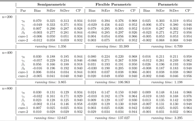
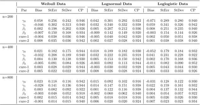
2.4 Simulation Studies . . . 30
2.6 Conclusions and Discussions . . . 46
Chapter 3 Semiparametric Estimation in the Population-level Promotion Time Cure Model . . . 48
3.1 Introduction . . . 48
3.2 Promotion Time Cure Model with Background Mortality . . . 50
3.3 EM Algorithm . . . 52
3.4 Simulation Studies . . . 58
3.5 Breast Cancer Data Analysis . . . 61
3.6 Discussions . . . 65
Chapter 4 Regression Analysis of Right-Censored Data Un-der the Generalized Odds-Rate Model . . . 68
4.1 Introduction . . . 69
4.2 Identifiability of GOR models . . . 71
4.3 The Proposed Method . . . 73
4.4 Simulation . . . 79
4.5 Real Data Analysis . . . 87
4.6 Discussions . . . 93
Bibliography . . . 95
Appendix A The quantities involved in var(θˆ) . . . 102
List of Tables
Table 1.1 Partial patients records in acute leukemia data . . . 3
Table 2.1 Summary Statistics for Weibull Data with Logistic Link: by semiparametric method, flexible parametric method with
mono-tone splines, parametric Weibull baseline function. . . 33 Table 2.2 Summary Statistics for Lognormal Data with Logistic Link: by
semiparametric method, flexible parametric method with
mono-tone splines, parametric Lognormal baseline function. . . 34 Table 2.3 Summary Statistics for Loglogistic Data with Logistic Link: by
semiparametric method, flexible parametric method with
mono-tone splines, parametric Loglogistic baseline function. . . 35 Table 2.4 Sensitivity Analysis: columns are Weibull, Lognormal and
Loglo-gistic data distributions; rows are the parametric Weibull, Log-normal, Loglogistic methods and the proposed semiparametric
method. . . 36 Table 2.5 Summary Statistics for the proposed semiparametric method
with logistic link (low cure rates) . . . 37 Table 2.6 SEER Louisiana regional female breast cancer: parameters
esti-mation in the semiparametric MCPH+BM model and the semi-parametric MCPH model, race and grade are included in both the cure logistic link function and latency survival function. Model I is to fit the whole data set with 6200 observations, Model II is to fit the subgroup of age ≤ 70 with 4267 obser-vations, and Model III is to fit the subgroup of age > 70 with
1933 observations. . . 42
Table 3.1 Summary Statistics for Weibull Data: by proposed semipara-metric method and parasemipara-metric method with Weibull baseline
Table 3.2 Summary Statistics for Lognormal Data: by proposed semipara-metric method and parasemipara-metric method with Lognormal baseline
function. . . 61 Table 3.3 Summary Statistics for Loglogistic Data: by proposed
semipara-metric method and parasemipara-metric method with Loglogistic baseline
function. . . 62 Table 3.4 Sensitivity Analysis for 800 Sample Size: rows represent
para-metric methods and semiparapara-metric method, and columns are
the Weibull, Lognormal and Loglogistic data. . . 63 Table 3.5 SEER regional female breast cancer: parameters estimation in
the semiparametric PCPH+BM model and the semiparametric PCPH model, race and grade are included in both the cure link function and latency survival function. Model I is to fit the whole data set with 6200 observations, Model II is to fit the subgroup data of age ≤ 70, and model III is to fit the subgroup data of
age >70. . . 64
Table 4.1 Summary Statistics of the proposed method with concave func-tion Λ0(t) = log(1 + t) + t1.5, β = c(−1,−1), ρ = 2, ρ = 1
and ρ = 0.5 with 3 levels censoring rate (around 20% in I: Low Censored, 40% in II: Medium Censored and 75% in III: High
Censored). . . 81 Table 4.2 Summary Statistics of the proposed method with convex
func-tion Λ0(t) = 0.5t5/6, β = c(−1,−1), ρ = 2, ρ = 1 and ρ = 0.5
with 3 levels censoring rate (around 20% in I: Low Censored,
40% in II: Medium Censored and 75% in III: High Censored). . . 82 Table 4.3 Summary Statistics of the proposed method with concave
func-tion Λ0(t) = log(1 +t) +t1.5,β =c(−1,−1) and in extreme cases
of ρ= 4 and ρ = 0.25 with 3 levels censoring rate (around 20% in I: Low Censored, 40% in II: Medium Censored and 75% in III: High Censored). Larger ρ provides larger frailty variance, and the setup underρ= 4 needs much larger sample size to provide
Table 4.4 Summary Statistics of the proposed method with convex func-tion Λ0(t) = 0.5t5/6, β = c(−1,−1) and in extreme cases of
ρ= 4 and ρ= 0.25 with 3 levels censoring rate (around 20% in I: Low Censored, 40% in II: Medium Censored and 75% in III: High Censored). Similar to the concave function Λ0(t), a larger
ρ provides larger frailty variance, and the setup under ρ = 4
needs much larger sample size to provide stable performance. . . . 84 Table 4.5 Summary Statistics for concave function Λ0(t) = log(1 +t) +t1.5,
β = c(−1,−1), ρ = 2 with 3 levels censoring rate (around 20% in I: Low Censored, 40% in II: Medium Censored and 75% in III: High Censored), the proposed EM algorithm performs much better than the direct MLE algorithm. In other settings, EM
algorithm also performs better and the results are not shown. . . . 85 Table 4.6 Power Analysis of the proposed method forρ = 1 (PO model).
Note the concave function is Λ0(t) = log(1 +t) +t1.5, convex
function is Λ0(t) = 0.5t5/6 and β =c(−1,−1). Sample size is 1500. 86
Table 4.7 Summary Statistics of the proposed method with fixed param-eter ρ, concave function Λ0(t) = log(1 +t) +t1.5, convex
func-tion Λ0(t) = 0.5t5/6, β =c(−1,−1) with 3 levels censoring rate
(around 20% in I: Low Censored, 40% in II: Medium Censored
and 75% in III: High Censored), and sample size of 200. . . 86 Table 4.8 SEER Louisiana Localized Lung Cancer Data: include sex, race
and grade in the survival function. Model I is to fit the data by estimating ρ with regression parameters, Model II fixes ρ = 0, and Model III fits the data with fixedρ = 1. The best number of interior knots is searched for 10, 15, 20 and 25 based on AIC
and BIC. . . 91 Table 4.9 SEER Louisiana Localized Lung Cancer Data: parameters
esti-mation in the proposed EM algorithm, sex, race and grade are included in the survival function. Interior knots are selected as
15 based on AIC and BIC for the three models. . . 92 Table 4.10 SEER Louisiana Localized Lung Cancer Data: parameters
esti-mation in the proposed EM algorithm, sex, race, grade and also the interaction of sex and race are included in the survival func-tion. Interior knots are selected as 15 based on AIC and BIC for
List of Figures
Figure 1.1 Kaplan Meier curve by race: the dark black line represents the survival probability for the black people and the light grey line
is the overall survival probability for the white people. . . 6 Figure 1.2 Stratified Kaplan Meier curve by Age 70: from light grey to
dark black successively are the overall survival probabilities for white of age ≤ 70, white of age > 70, black of age ≤ 70 and
black of age >70. . . 6
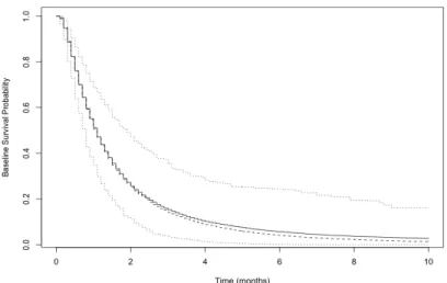
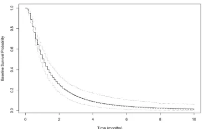
Figure 2.1 Baseline Survival Probability Estimation for Weibull Data by
Semiparametric MCPH+BM Model (200 Sample Size). . . 35 Figure 2.2 Baseline Survival Probability Estimation for Weibull Data by
Semiparametric MCPH+BM Model (400 Sample Size). . . 36 Figure 2.3 Baseline Survival Probability Estimation for Weibull Data by
Semiparametric MCPH+BM Model (800 Sample Size). . . 37 Figure 2.4 Baseline Survival Probability Estimation for Lognormal Data
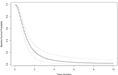
by Semiparametric MCPH+BM Model (200 Sample Size). . . 38 Figure 2.5 Baseline Survival Probability Estimation for Lognormal Data
by Semiparametric MCPH+BM Model (400 Sample Size). . . 38 Figure 2.6 Baseline Survival Probability Estimation for Lognormal Data
by Semiparametric MCPH+BM Model (800 Sample Size). . . 39 Figure 2.7 Baseline Survival Probability Estimation for Loglogistic Data
by Semiparametric MCPH+BM Model (200 Sample Size). . . 39 Figure 2.8 Baseline Survival Probability Estimation for Loglogistic Data
by Semiparametric MCPH+BM Model (400 Sample Size). . . 40 Figure 2.9 Baseline Survival Probability Estimation for Loglogistic Data
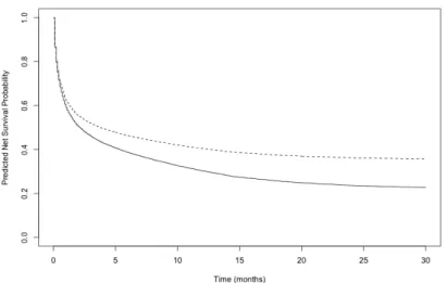
Figure 2.10 Predicted Net Survival Probability for the Simulated Data of 200 Sample Size Weibull Distribution: dashed line and solid line represent the predicted survival probabilities for treatment
and control arms respectively. . . 41 Figure 2.11 Predicted Net Survival Probability for the Simulated Data of
200 Sample Size Lognormal Distribution: dashed line and solid line represent the predicted survival probabilities for treatment
and control arms respectively. . . 41 Figure 2.12 Predicted Net Survival Probability for the Simulated Data of
200 Sample Size Loglogistic Distribution: dashed line and solid line represent the predicted survival probabilities for treatment
and control arms respectively. . . 42 Figure 2.13 The MCPH+BM model predicts the net survival probability by
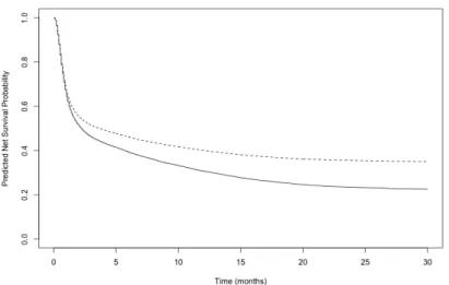
race, and the MCPH model predicts the observed (net) survival
probability by race. . . 44 Figure 2.14 Predicted net survival under the MCPH+BM model and the
MCPH model for the subgroup of Age > 70 in the SEER
re-gional female breast cancer. . . 44 Figure 2.15 Predicted net survival under the MCPH+BM model and the
MCPH+BM model for the subgroup of Age ≤70 in the SEER
regional female breast cancer. . . 45 Figure 2.16 Pseudo Data Estimation Output by the R Package “psmcur” . . . 45
Figure 3.1 Predicted Survival Probability for the SEER regional female breast cancer data, the proposed PCPH+BM model estimates
cure fraction higher than the standard PCPH model. . . 64 Figure 3.2 Predicted Survival Probability for the subgroup of age ≤ 70
in the SEER regional female breast cancer data. The proposed PCPH+BM model estimates cure fraction higher than the
stan-dard PCPH model. . . 65 Figure 3.3 Predicted Survival Probability for the subgroup of age > 70
in the SEER regional female breast cancer data. The proposed PCPH+BM model estimates cure fraction higher than the
Figure 4.1 Case i: Solid line is the estimated Λ01(t) and dashed line is the
estimated Λ02(t). . . 72
Figure 4.2 Case ii: Solid line is the estimated Λ01(t) and dashed line is the
estimated Λ02(t). . . 73
Figure 4.3 Estimated baseline survival probability for the concave function Λ0(t) = log(1 +t) +t1.5,β =c(−1,−1), ρ= 2 with low censored
rate (sample size 200). . . 87 Figure 4.4 Estimated baseline survival probability for the concave function
Λ0(t) = log(1 +t) +t1.5,β =c(−1,−1), ρ= 2 with low censored
rate (sample size 500). . . 87 Figure 4.5 Estimated baseline survival probability for the concave function
Λ0(t) = log(1 +t) +t1.5,β =c(−1,−1), ρ= 2 with low censored
rate (sample size 1000). . . 88 Figure 4.6 Estimated baseline survival probability for the concave function
Λ0(t) = log(1 +t) +t1.5,β =c(−1,−1), ρ= 2 with low censored
rate (sample size 1500). . . 88 Figure 4.7 Estimated baseline survival probability for the concave function
Λ0(t) = log(1 +t) +t1.5, β = c(−1,−1), ρ = 2 with medium
censored rate (sample size 200). . . 89 Figure 4.8 Estimated baseline survival probability for the concave function
Λ0(t) = log(1 +t) +t1.5, β = c(−1,−1), ρ = 2 with medium
censored rate (sample size 500). . . 89 Figure 4.9 Estimated baseline survival probability for the concave function
Λ0(t) = log(1 +t) +t1.5, β = c(−1,−1), ρ = 2 with medium
censored rate (sample size 1000). . . 90 Figure 4.10 Estimated baseline survival probability for the concave function
Λ0(t) = log(1 +t) +t1.5, β = c(−1,−1), ρ = 2 with medium
censored rate (sample size 1500). . . 90 Figure 4.11 Predicted survival probability vs. Time (years) for White
Fe-male and White Male in the SEER Localized Lung Cancer Data under the proposed method and compared to the Kaplan Meier Curve. The proposed method predicts the survival probability
Figure 4.12 Predicted survival probability vs. Time (years) for Black Fe-male and Black Male in the SEER Localized Lung Cancer Data under the proposed method and compared to the Kaplan Meier Curves. The proposed method predicts the survival probability
Chapter 1
Introduction
1.1 Survival Data
Survival analysis is a collection of statistical procedures that study the duration of time until one particular event of interest happens and thus it is also called time-to-event analysis. The survival time can be years, months, weeks or days from the beginning of follow-up of an individual until the event of interest occurs. The event of interest can be death, disease incidence, relapse from remission or recovery from disease that may happen to a patient. For example, if the event of interest is death, then the survival time will be the time in years until a patient dies. However, the survival time may not be observed directly in some cases. In some studies especially in clinical trial studies, patients are examined only at discrete observational times, and the statuses whether the patients have experienced the event of interest or not at these observational times can be recorded. However, the event time may not be known exactly but be known to fall within some time interval. In other studies, some patients may not experience the event of interest by the end of a study, or some patients have already experienced the event of interest before being recruited in a study. All these phenomena are called censoring, where some survival time of interest can not be known exactly.
Censoring occurs when we have some information about subjects’ survival time, but we do not know what are their exact survival time. Thus censoring is a condition in which a subject’s survival time is only partially known. For example, a patient
moves to another state after being recruited to a clinical trial and is lost to be traced. The only information available on his or her survival time is the last date on which this patient was known to be alive. This date may be the last time that this patient reported to a clinic for a regular check-up.
There are various categories of censoring, such as right censoring, left censoring, and interval censoring. Right censoring occurs when a subject’s exact survival time is not observed and is known to be greater than this person’s observation time. Left censoring occurs when a subject’s exact survival time is less than or equal to this person’s observation time. Interval censoring means a subject’s exact survival is only known to lie within an interval instead of being observed directly. Below are some real life examples to illustrate different censored data.
1.1.1 Right-Censored Data
The Acute Leukemia Group (1963) has reported the results of a clinical trial of a drug 6-mercaptopurine (6-MP) versus a placebo in twenty-one pairs of patients with acute leukemia. This trial was conducted at eleven American hospitals. Patients who had a complete or partial remission of their leukemia induced by treatment with the drug prednisone were selected. A complete or partial remission means that either most or all signs of disease had disappeared from the bone marrow.
The trial was conducted by matching pairs of patients at a given hospital by remission status (complete or partial) and randomizing within the pair to either a 6-MP or placebo maintenance therapy. Patients were followed until their leukemia relapsed or until the end of the study. The event of interest is the relapse of leukemia and the survival time is the time in weeks until patients went out of remission.
Part of the patients records are shown in table 1.1. Patient A was followed from the start of the study until getting leukemia relapsed at week 5, so this person’s survival time was observed to be 5 weeks. Patient B was observed from the start
Table 1.1: Partial patients records in acute leukemia data Patient Enter Time End Time Reason Failed(1); censored (0)
A 0 5 out of remission 1 B 0 12 study ends 0 C 2.5 6 withdrawn 0 D 4 12 study ends 0 E 3 9 lost to follow up 0 F 8 11.5 out of remission 1
of the study, but did not experience the relapse until the end of the 12-week study period, so this person’s survival time was censored and at least 12 weeks. Patient C entered the study between week two and week three and was followed until he or she withdrew at week 6, so this person’s survival time was censored. Patient E entered the study at week 3 and was lost to follow at week 9, so this person’s survival time was censored and at least 6 weeks. In summary, the patient A and F experienced leukemia relapse and their survival times are known exactly. The other four patients did not experience leukemia, and thus their survival times are right-censored. This data set is an example of right-censored data in the survival literature, which contain some exactly observed survival times and some right-censored survival times.
1.1.2 Left-Censoring Data
One example is that in early childhood learning centers, research interest often focuses upon testing children to determine when a child learns to accomplish certain specified tasks such as reciting the alphabet. The age at which a child can recite the alphabet would be considered as the time-to-event. Often, some children are already able to recite the alphabet when they are recruited in the study. Such survival times are considered left-censored.
Another example is on clinical trial studies. Human immunodeficiency virus (HIV) is a chronic disease which weakens the immune system. HIV RNA or viral load (VL) measures the number of actively replicating HIV virus in a subject, which is an important biomarker for HIV disease. The suppression of VL to undetectable
levels can improve physical functioning and reduce HIV related mortality. VL is undetectable if it has less than 200 copies of HIV per milliliter of blood by the CDC guideline. In a study of the HIV, the observations start from the time points when patients’ VL reach detectable levels. However, the exact survival time that some subjects’ VL reach detectable levels are unknown and these survival times are left-censored.
1.1.3 Interval-Censored Data
De Gruttola and Lagakos (1989) discussed the study involving a cohort of hemophil-iacs for whom both infection with the HIV and the onset of the acquired immunode-ficiency syndrome (AIDS) or other clinical symptoms. The data were collected from 262 patients with type A or B hemophilia in France between 1978 and 1988. Twenty-five of the patients were detected to be infected with HIV on their first lab tests. By August 1988, 197 hemophiliacs had been infected and 43 of these showed the acqui-sition of AIDS or other clinical symptoms such as lymphadenopathy or leukopenia. These patients were believed to become infected from the infusions of contaminated blood factor they received periodically to treat their hemophilia. Blood were pe-riodically sampled and stored to decide a time interval during which the infections occurred. Thus, the infection times were censored within a time interval with changed status from negative to positive.
1.2 Motivating Data
Right-censored data are the most common type of censored data in oncology studies and cancer statistics. In these studies, the time-to-event is usually the survival time until death. In this dissertation, we focus on analyzing right-censored data in different survival models. The data for illustration are from the Surveillance, Epidemiology, and End Results Program (SEER) (Howlader et al., 2019). The SEER cancer data
is the research data from population-based cancer registries covering approximately 34.6 % of the United States population. The SEER registries collect data on patient demographics, primary tumor site, tumor morphology, stage at diagnosis, and first course of treatment, and they follow up with patients for vital status. The vital status is recorded as dead or alive.
Breast Cancer Data
Breast cancer is fairly common in female, representing about 15.2% of all new cancer cases in the United States. Female breast cancer is the fourth leading cause of death in the United States, and it is most frequently diagnosed among women aged 55-64. Women who are diagnosed at older age may be more likely than younger women to die of the disease, and family history increases the risk of breast cancer (Howlader et al., 2019). Regional breast cancer, which is defined as cancer cells spread to regional lymph nodes, accounts for 30% of all the cases by stage. The 5-year relative survival probability for regional breast cancer is 85.5%. For illustration, we use the SEER Louisiana regional female breast cancer for patients of age > 50 with the diagnosis year between 2000 to 2012 (Howlader et al., 2019).
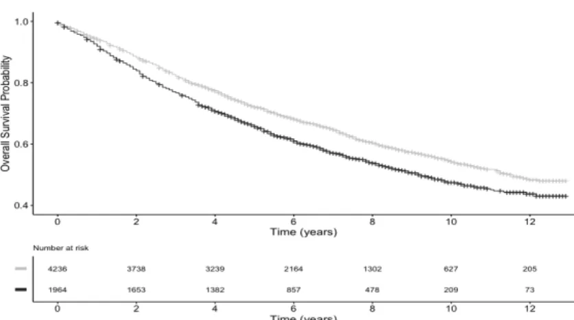
A total of 6200 patients were included in this study with a mean age at diagnosis of 65.7 years old, a censoring rate of 59.5% and a maximum follow-up time of 12.9 years. 1933 patients (31.2%) were older than 70 years old, 4236 patients (68.3%) are white, and 1964 patients (31.7%) are black. There are also other races in this data set, but we focus on the comparison between the white people and the black people. Figure 1.1 shows that there is a significant difference in survival probability be-tween the white and the black with the log-rank test p-value= 6e-08. We further illustrate the Kaplan Meier curve stratified by each race and age (> 70 and ≤ 70) group in Figure 1.2, which indicates the survival probabilities also vary by age groups. The four subgroups including white and age > 70, black and age > 70, white and
Figure 1.1: Kaplan Meier curve by race: the dark black line represents the survival probability for the black people and the light grey line is the overall survival proba-bility for the white people.
Figure 1.2: Stratified Kaplan Meier curve by Age 70: from light grey to dark black successively are the overall survival probabilities for white of age ≤ 70, white of age
>70, black of age≤70 and black of age>70.
age ≤ 70 and black and age ≤70 have significant different survival probabilities (p-value=2e-16). It is worthwhile pointing out that in this data set, the event of interest is the record of vital status of either being dead or alive, so the enrolled patients may die from causes other than breast cancer, especially for elderly patients who may die from aging. Those deaths from other causes can obscure the accurate estimation of survival probability and cure fraction, because those patients dying from other causes may also benefit from the treatment of breast cancer.
Lung Cancer Data
From the SEER 1975-2016 Research Database (Howlader et al., 2019), we also select a subset of the data for the Louisiana localized lung cancer study. This data set contains subjects aged at least 50 from the state of Louisiana whose diagnosis year is between 2004 to 2016. The response variable of interest is the time to death since diagnosis, for which right-censored data are available since not all patients died by 2016. Our data set only focuses on the data from white and black races although there are many other races in the original data set.
In total, there are 9,965 observations in this data set, and the right-censored rate is 42.76%. We consider three covariates of interest: “sex” taking 1 for female and 0 for male, “race” taking 1 for black race and 0 for white race, and “grade”, which is a measurement of how closely the tumor cells resemble lung ranging from 1 to 9 representing different degrees of differentiation.
1.3 Survival Models
For the past decades, survival analysis has been adapted for application in different areas such as biology and biomedical studies. We denote by T the random variable for a subject’s survival time, which is a non-negative continuous variable. We also denote by t any specific value of interest for the random variableT. For example, if we are interested in studying whether a patient survives for more than 5 years after undergoing cancer therapy, then t= 5. Specifically for right-censored data, let Y be the observation time of patients and C denote their censoring time. Let δ denote a random variable with possible values 0 and 1 which indicates either censoring or failure. That is,δ = 1 for failure if the event of interest occurs during a study, orδ = 0 if the survival time is censored by the end of a study. We have Y =T if a subject’s exact survival time is observed and Y =C if it is censored, i.e., Y = min(T, C) and
The cumulative distribution function of T isF(t) = P(T ≤t) and its correspond-ing probability density function is denoted asf(t). The survival function of T is the probability that a subject survives longer than some specified timet, given by
S(t) =P(T > t) = 1−F(t) =
Z ∞ t
f(s)ds,0< t <∞.
The survival functions are nonincreasing and head-downward as t increases. At time
t= 0, S(t) = S(0) = 1.
The hazard function gives the instantaneous potential per unit time for the event of interest to occur given that the subject has survived up to timet, which is expressed as
λ(t) = lim
∆t→0
P(t≤T < t+ ∆t|T ≥t)
∆t .
The relationship between survival function S(t) and hazard function λ(t) is
λ(t) = f(t) S(t) =− dlogS(t) dt and S(t) = exp{− Z t 0 λ(s)ds}= exp{−Λ(t)},
where Λ(t) is the cumulative hazard function until time t.
Below are some popular survival models which are used to estimate the effect of potential covariates on the survival time of patients.
1.3.1 the Proportional Hazards Model
One of the most important statistical models in survival analysis is the proportional hazards (PH) model proposed by Cox (1972). The PH assumption introduces covari-ates into the model and specifies the hazard function in the following form,
h(t|x) =h0(t) exp(β|x),
where h(·|x) is the hazard function with covariates x, h0(·) is the baseline hazard
proportional hazards with respect of the covariates x such that the hazard ratio for individuals with x1 and x2 is exp{β|(x1−x2)}, which is constant over time.
Therefore, the Cox PH model essentially assumes that the treatment effect is constant over time. The cumulative hazard function in the PH model is the integral of baseline hazard function, defined as H(t|x) = R∞
0 h(t|x)dt, and the logarithm of cumulative
hazard function is expressed as
log{H(t|x)}=β|x+ log{H0(t)},
which shows that the curves log{H(t|x)} for different values ofx are parallel. For estimation in the PH model, Cox (1975) proposed the partial likelihood to estimate parametersβwithout involving the baseline functionh0(t), which is the most
popular estimation approach in survival analysis for right-censored data. Suppose we observe (Yi, δi, xi) for individual i = 1, . . . , n, where Yi is a observed failure time
random variable, δi is the failure/censoring indicator (1=failure, 0=censoring), and
xi represents a vector of covariates. Assume that there are K distinct failure times
and there are no ties among these event times. Let t(1) < t(2) <· · ·< t(K) represent
the K ordered distinct failure times, and x(i) is the covariates for the subject that
has the failure at time t(i). Let R(t) = {i : Yi ≥ t} denote the at-risk set at time t,
the partial likelihood for the Cox PH model is
L(β) = K Y i=1 exp{β|x (i)} P j∈R(ti)exp (β |x j) . (1.1)
The partial maximum likelihood estimator of β is found by solving the partial likelihood score equation obtained by setting the derivative of the partial likelihood (1.1) with respect toβ to 0 in the following form
K X i=1 x(i)− K X i=1 P j∈R(ti)xjexp (β |x j) P j∈R(ti)exp (β |x j) = 0.
1.3.2 the accelerated failure time model
While the Cox PH model specifies that the effect of covariates is multiplicative with respect to the hazard, the accelerated failure time (AFT) models are that the effect of covariates is multiplicative or proportional with respect to survival time. The survival time T in the AFT models maintain the following relationship with covariates
logT =β|x+,
where x is a vector of covariates and are independent random errors. Different parametric distributions can be assumed forto generate different survival functions. Maximum likelihood estimation can be applied in the AFT models.
1.3.3 the proportional odds model
When the effect of covariates diminishes over time in two-sample cases, one possibility is to use time-dependent covariates in the Cox PH model. Alternatively, one may use the proportional odds (PO) model (Bennett, 1983a). The PO model assumes that the odds ratio remains constant over time. The odds ratio is the ratio of failure odds of getting the event by timet for different groups, and the failure odds is denoted by
F(t)/1−F(t). The PO model specifies that given covariate x, the odds for survival at timet is F(t|x) 1−F(t|x) = F0(t) 1−F0(t) exp (β|x),
where F0(t) is an unknown baseline cumulative distribution function. The hazard
function given xis λ(t|x) = exp (β |x) exp (β|x)R(t) + 1 dR(t) dt ,
where R(t) = F0(t)/(1−F0(t)). Hence for two different sets of covariates x1 and x2,
1.3.4 the generalized odds-rate model
The generalized odds-rate (GOR) models was proposed by Harrington and Fleming (1982) and its survival function is expressed as
S(t|x) = {1 +ρΛ0(t) exp(β|x)}−ρ
−1
, t >0. (1.2)
In the GOR survival function, Λ0(t) is a strictly positive increasing function, β
is a p× 1 vector of regression parameters denoting the covariate effects and ρ is a positive constant. Specifically, as ρ → 0, equation (1.2) has a limiting survival functionS(t|x) = exp{−Λ0(t)}
exp (β|x)
=S0(t)exp (β
|x)
, which is the survival function under the Cox PH model. Whenρ= 1, equation (1.2) becomes the PO model survival function S(t|x) = {1 + Λ0(t) exp (β|x)}−1.
Previous studies in the GOR models are mainly focused on estimating regression parameters β by fixing the parameter ρ and selecting model by Akaike information criterion (AIC) or Bayesian information criterion (BIC), for example, in Cheng, Wei, and Ying (1995); Cheng, Wei, and Ying (1997); Scharfstein, Tsiatis, and Gilbert (1998); Fine, Ying, and Wei (1998); Slud and Vonta (2004); Dabrowska (2006) and Yin and Zeng (2006), among others. The regression parametersβ and the increasing function Λ0(t) can be estimated by maximum likelihood estimation.
1.3.5 Cure Models
Although the Cox PH model and the partial likelihood estimation approach are widely used due to its fast computation and easy interpretation. In practical circumstances, the proportional hazards assumption may not be satisfied.
With the rapid development of medication, more and more diseases and even cancers are curable in the long run such as breast cancer and colon cancer, thus, there is a proportion of patients may never experience the event of interest for a long time. The Kaplan-Meier curve will level off and reach a plateau at the end of the
study to indicate the cure. The classic cure models are used to address this issue, and two commonly adopted cure models are the mixture cure model and the promotion time cure model.
Mixture Cure Model
The mixture cure model was first proposed by Berkson and Gage (1952) and previous research in literature include Gray and Tsiatis (1989), Kuk and Chen (1992), Sy and Taylor (2000), Peng and Dear (2000), Betensky and Schoenfeld (2001), Lambert (2007), Cai et al. (2012), Ortega et al. (2014) among others. The mixture cure model is expressed as
Spop(t|x,z) =π(z)S(t|x) + 1−π(z), (1.3)
where 1−π(z) is the probability of the subjects being cured depending on the co-variates z, and S(t|x) is referred to as a latency survival function, which is the survival probability of the uncured patients depending on the covariates x. Note that π(z) can take different link functions such as the logit link function π(z) = exp (γ|z)/{1 + exp (γ|z)}, the log-log link function logh−log{1−π(z)}i, and the probit link function Φ−1{π(z)}=γ|z, where Φ(·) is the cumulative distribution func-tion of standard normal distribufunc-tion. If the PH model is used to model the latency survival functionS(t|x), the mixture cure model is called the mixture cure PH model.
Promotion time cure model
The promotion time cure model was initially motivated by a biological model to analyze the time-to-relapse in cancer studies (Andrei and Asselain, 1996; Tsodikov, 1998 Chen, Ibrahim, and Sinha, 1999; Tsodikov, Ibrahim, and Yakovlev, 2003; Yin and Ibrahim, 2005). For ith individual with covariates zi, the survival function for
individuali is given by
where θ(·) is a link function and F(t) is a latency cumulative distribution function. The corresponding latency survival function is denoted by S(t) = 1− F(t), and the latency probability density function is f(t) = dF(t)/dt. The cure fraction is
Spop(∞|zi) = exp{θ(zi)} when time goes to infinity, and the cure fraction is always
positive. The promotion time cure model is strongly motivated by biological con-siderations of tumour cells. For the patient i, let Ni be the number of tumour cells
which have the potential of metastasizing (metastasis-competent tumour cells), and it is assumed thatNi has a Poisson distribution with meanθ(zi). The promotion time
for the kth (k = 1, . . . , Ni) tumour cell is denoted as ˜Tk, which is the time for the kth metastasis-competent tumour cell to produce a detectable tumour mass. Assume that ˜Tk’s are independent and identically distributed with the cumulative distribution
function of F(t) conditional on Ni. Note that both Ni and ˜Tk are unobserved latent
variables which can be explored by Expectation-Maximization (EM) algorithm. The time to relapse of cancer is defined as Ti = min( ˜T1, . . . ,T˜Ni). The survival function
can be further written as
Spop(t|zi) = P(Ti > t) =P(Ni = 0) + X k≥1 P( ˜T1 > t, . . . ,T˜Ni > t|Ni =k)P(Ni =k) = exp{−θ(zi)}+ ∞ X k=1 S(t)kθ(zi) kexp{−θ(z i)} k! = exp{−θ(zi)F(t)}. (1.5)
The corresponding hazard rate for the subjecti isθ(zi)f(t) and the link function θ(zi) usually takes the exponential form exp(γ|zi). To be consistent with (1.3) in the
mixture cure model, (1.5) is also to allowF(t) to depend on a vector of covariatesxi,
leading to
Spop(t|zi,xi) = exp{−θ(zi)F(t|xi)}. (1.6)
The mixture cure model and promotion time cure model are the most widely used cure fraction models in application and each has its own advantages as well as
draw-backs as discussed in Chen, Ibrahim, and Sinha (1999) and Ibrahim, Chen, and Sinha (2001). The mixture cure model is more straightforward to interpret since it involves two parts to indicate cured and uncured patients. From the Bayesian perspective, when a uniform improper prior is set for the parametersγ, the posterior distribution forγ is proper only in the promotion time cure model but is improper in the mixture cure model. When including the covariates z through the link function for π via a standard binomial regression model, (1.3) yields improper posterior distributions for many types of noninformative improper priors, including the uniform prior.
1.4 Existing Regression Approaches
There are many new emerging approaches proposed in the past decades for analyzing right-censored data, and the ultimate goal is to estimate the covariate effects on the survival time. Parametric models work well only when the distribution of baseline functions are correctly specified, but semiparametric regression models are more pre-ferred in application since they would avoid the problem of misspecification and gain much modeling flexibility.
The partial likelihood function in equation has eliminated the infinite dimen-sional baseline hazard function from the estimation of regression parameters for right-censored data. Andersen and Gill (1982) established the asymptotic properties of the maximum partial likelihood estimator. Breslow (1972) proposed the nonparamet-ric estimator for cumulative baseline hazard function via counting process martingale theory. This type of estimator is called nonparametric maximum likelihood estimator (NPMLE). When the proportional hazards assumption is violated, Bennett (1983b) proposed a semiparametric maximum likelihood estimator (MLE) for estimating the regression parameters in the PO model. Parzen and Harrington (1993) used adaptive splines with small number of knots to estimate baseline odds of failing by time. The
NPMLE based on the profile likelihood function was studied in Murphy, Rossini, and Vaart (1997).
For the more generalized GOR models, Cheng, Wei, and Ying (1997) proposed a semiparametric approach to estimate the regression parameters. Scharfstein, Tsiatis, and Gilbert (1998) studied the NPMLE for the regression parameters conditional on
ρ being fixed and known. Chen, Jin, and Ying (2002) developed simple martingale-based estimating equations to estimate regression parameters. The theoretical prop-erties and hypothesis tests of the NPMLE for general transformation models have been studied by Bagdonavicius and Nikulin (1999), Kosorok, Lee, and Fine (2004), Zeng and Lin (2006) and Song, Kosorok, and Fine (2009).
For the cure models estimation, parametric models and flexible parametric mod-els usually adapt Newton-Raphson algorithm to maximize the observed likelihood function. In semiparametric cure models, EM algorithm is used to estimate parame-ters and cure fraction. The EM algorithm was first introduced by Dempster, Laird, and Rubin (1977) (DLR). The DLR paper makes significant contributions such that it recognizes the expectation step (E-step) and the maximization step (M-step), it gives theoretical properties of the EM algorithm and it also provides a wide range of applications in statistics. The EM algorithm has become a very popular com-putational method in statistics for both frequentists and Bayesian approaches. The implementation of the E-step and M-step is easy for many statistical problems and even for complex models. The M-step can be performed by existing R packages such as “optim” or “nleqslv” which makes the algorithm more computationally efficient. Moreover, the EM algorithm does not require large storage space. Louis (1982) pro-posed the observed information matrix for the EM algorithm, and it provides the variance estimation in closed form which makes the EM algorithm even more appeal-ing.
The most crucial deterrent in the MLE is the potentially unlimited dimension in semiparametric regression models. The Newton-Raphson method in maximizing the full likelihood function requires O(d3) (d is the number of parameters) operations
to solve a system of score equations. The principal part of the d parameters in a semiparametric regression model is to specify a stepwise function H which may approach the true continuous function as d goes to infinity. A large d will make the maximization by Newton-Raphson method has high complexity and is very difficult in computation. On the contrary, the EM algorithm handles the H function in an
O(d) way.
The EM algorithm can be extended to involve a profile likelihood, such that the E-step involves computation of the expectation of full likelihood function with respect to the observed data, and the M-step is to estimate covariate effects using the profile likelihood in Johansen (1983). Let θ = (β, H), where β is a vector parameters of interest and H is the stepwise function of a nuisance vector parameters. We denote
O as the observed data. The profile likelihood of β is the likelihood function defined as
Lp(β;O) = supHL(β,H;O).
1.5 Structure of the Dissertation
The rest of the dissertation is structured as follows. In Chapter 2, we will study the mixture cure PH model with background mortality (MCPH+BM) and its com-putational estimation approach. An EM algorithm with latent variables to indicate uncured status is developed to estimate the semiparametric MCPH+BM model, and a perturbation variance estimation method is also discussed. The implementation of R functions in the “psmcure” package published in Github is further described. The results of comprehensive simulation studies and a real data application are provided to evaluate the performance of the proposed method. In Chapter 3, we propose an
EM algorithm to estimate cure fraction in the promotion time cure PH model with background mortality (PCPH+BM). The simulation studies show that the proposed semiparametric method is robust to different data distributions. A real data exam-ple is provided to illustrate the proposed method and compare the estimation to the case when background mortality is ignored. A generalization of transformation model with background mortality is further considered. In Chapter 4, we discuss the identi-fiability problems in the GOR models and propose a novel EM algorithm to estimate all the regression parameters and the parameter ρ simultaneously.
Chapter 2
Semiparametric Estimation of the Cure
Fraction in Population-based Cancer Survival
Analysis
Abstract
With rapid development in medical research, the treatment of diseases including can-cer has progressed dramatically and those survivors may die from causes other than the one under study, especially among elderly patients. Motivated by the SEER female breast cancer study, background mortality is incorporated into the mixture cure proportional hazards (MCPH) model to improve the cure fraction estimation in population-based cancer studies. Here, that patients are “cured” is defined as when the mortality rate of the individuals in diseased group returns to the same level as that expected in the general population, where the population level mortality is pre-sented by the mortality table of the United States. The semiparametric estimation method based on the EM algorithm for the MCPH model with background mortality (MCPH+BM) is further developed and validated via comprehensive simulation stud-ies. Real data analysis shows that the proposed semiparametric MCPH+BM model may provide more accurate estimation in population-level cancer study.
2.1 Introduction
The treatment of diseases including cancer has progressed dramatically and results in a high survival probability. The 5-year relative survival probability is as high as 98.2% for thyroid cancer, 98.0% for prostate cancer, 89.9% for female breast cancer, and 64.4% for colorectal cancer from the Surveillance, Epidemiology, and End Results (SEER) Program (2009-2015) (Howlader et al., 2019). In the long follow-up time, those survivors may die from causes other than the one under study, especially in the case of many elderly patients in a study (Verheul et al., 1993), which may obscure the estimation of survival probability of interest.
Relative survival is a net survival measurement representing cancer survival in the absence of other causes of death. It helps to evaluate heath care effectiveness for the whole population or segments of the population. Relative survival was proposed by Esteve et al. (1990) such that observed survival probability is the product of corrected survival probability and expected survival probability, and observed hazard rate is the sum of corrected hazard rate and excess hazard rate. Previous studies are mainly focused on how to model the excess hazard. Giorgi et al. (2003) developed a B-splines relative survival regression model to model hazard ratios. Dickman et al. (2004) pro-posed a generalized linear model to estimate additive hazards. Stare, Pohar, and Henderson (2005) addressed the goodness of fit problem of relative survival model. Pohar and Stare (2006) developed a R package “relsurv” to apply several relative survival regression models. Nelson et al. (2007) proposed a model restricted cubic splines on the log cumulative excess hazard scale to estimate the relative survival and excess mortality rates. Perme, Henderson, and Stare (2008) used EM algorithm by treating the cause of death as missing data which is a generalization of the Cox PH model and provides flexibility in baseline excess hazard estimation and they fur-ther proposed a new estimator of net survival probability that enables comparability between countries.
A similar situation that patients may suffer from other events is competing risk (CR), which is an event either hinders the observation of the event of interest or alters its probability of occurrence (Gooley et al., 1999). The information from CR event is needed to derive the subdistribution function and marginal function of the event of interest. When the event of interest is death, the main difference between relative survival and competing risk rests on whether the other causes of death are known. In this paper we consider the case when death is all-cause death rather than causes-specific death, therefore the relative survival model is more appropriate. We propose the cure fraction estimation with background mortality based on the structure of relative survival.
Cure models have been employed to analyze cancer studies with potentially cured patients. In the standard cure models, “cure” is defined as patients will never ex-perience the event of interest in the future with a probability of one (Boag, 1949). The standard mixture cure model is for the case when the specific cause of death is recorded, so death is disease-related death. In competing risk, at least two causes of death are known and included in the analysis. However, when the cause of death is unknown or not recorded, the influence of mortality due to other causes should be incorporated. De Angelis et al. (1999) proposed the new definition of “cure” in a population level, that is, the mortality risk of cured patients will return to the similar mortality risk as their counterpart in the general population, which is referred to as background mortality. The mixture cure model with background mortality which incorporates the mortality of general population is more appropriate to this type of studies than the standard mixture cure model, since it accounts for the mortality due to other causes (Lambert et al., 2006). Thus, it can improve accuracy in estimat-ing the survival probability of uncured patients and cure fraction. The background mortality can be defined via a population-level life table with matched sex and age.
De Angelis et al. (1999) incorporated the background mortality into the mixture cure proportional hazards (MCPH) model under the exponential and Weibull distri-butions for uncured patients. Phillips, Coldman, and McBride (2002) extended De Angelis’s model to estimate the prevalence of cancer. Sposto (2002) described three link functions for the cure fraction estimation. Lambert et al. (2006) incorporated the background mortality to the parametric Weibull cure model via Newton-Raphson algorithm which is implemented in STATA (Lambert, 2007). They (Lambert et al., 2010) also have proposed a finite mixture of Weibull distributions to add flexibility, which also adds the complexity of estimating more Weibull parameters. Royston and Lambert (2011) discussed different topics such as time-dependent and continuous covariates in relative survival. Andersson et al. (2011) proposed to use flexible para-metric survival model with cubic splines to estimate cure fraction in population-based studies, which however do not allow covariates included in cure fraction function. All these previous studies on cure model with background mortality used maximum like-lihood function to estimate parameters and cure fraction.
Even though there are discussions on semiparemetric estimation methods of the MCPH model (Cai et al., 2012; Peng and Dear, 2000), few work is available in the literature on the semiparametric estimation method for the MCPH model with back-ground mortality. In addition, it is well understood that there are limitations in parametric and flexible parametric estimations, because the appropriate parametric distribution is hard to specify and the number of knots and degree of splines have to be selected. The purpose of this paper is to fill the gap in the study of semiparametric estimation method in the mixture cure model with background mortality. The rest of the paper is organized as follows. Section 2.2 illustrates the MCPH model with background mortality (MCPH+BM). The semiparametric estimation method are de-scribed in Section 2.3. Section 2.4 outlines the simulation studies and Section 2.5 applies the proposed method to the real data. Section 2.6 provides some conclusions.
2.2 Mixture Cure Model with Background Mortality
Similar to the mixture cure model, the mixture cure model with background mortality has two components:
1. patients being cured, whose mortality risk will return to the similar mortality risk level as their counterpart in the general population;
2. uncured patients, who will not only have the risk of death from disease of interest, but also suffer from the similar mortality risk as their counterpart in the general population.
Let t denote failure time, h∗(t) and S∗(t) are the population-level hazard risk which is also called background mortality rate, and the corresponding background survival probability as their counterpart in the general population with matched sex and age. Denote hu(t) and Su(t) as the hazard rate of the disease of interest and the
corresponding survival probability. For cured patients, the hazard rate is h∗(t) with survival probability ofS∗(t); for uncured patients, the hazard risk ish∗(t)+hu(t) with
survival probability of S∗(t)Su(t). Let us assume the proportion of cured patients is
indicated by (1−π). The mixture cure model with background mortality is expressed as
Spop(t) =πS∗(t)Su(t) + (1−π)S∗(t).
The corresponding population-level hazard function is expressed as
hpop(t) =h∗(t) +
πfu(t) πSu(t) + 1−π
,
where fu(t) is the probability density function associated with the survival function Su(t). Note, the model reduces to the standard mixture cure model whenS∗(t) = 1 or h∗(t) = 0, which is the mixture cure model ignoring background mortality risk. The second component in the population-level hazard function πfu(t)/{πSu(t) + 1−π}
is the corresponding hazard function for the standard mixture cure model. The hazard function of the mixture cure model with background mortality is intuitively the summation of the background hazard rate and the disease-related hazard rate.
Let z denote a vector of covariates, which may impact the uncured fraction, and the model turns to the mixture cure model with background mortality (Lambert et al., 2006; Lambert, 2007) such that
Spop(t) = S∗(t){π(z)Su(t) + 1−π(z)}, (2.1)
where π(z) can be modeled via the logistic link, log-log link or probit link. Let x denote a vector of covariates having potential effects on the latency survival func-tion Su(t). It is worthwhile pointing out that the same covariates are allowed for
x and z although we use different covariate notations, which is more flexible than existing methods. When Su(t) is specified via the proportional hazards assumption
ofSu(t|x) =S0(t)exp(β
|x
i), equation (2.1) turns to the MCPH model with background
mortality (MCPH+BM) (De Angelis et al., 1999; Royston and Lambert, 2011), which is written as
Spop(t) = S∗(t){π(z)S0(t)exp(β
|x
i)+ 1−π(z)}.
Similarly, as S∗(t) = 1 or h∗(t) = 0, equation (2.1) reduces to the standard MCPH model.
Let Oi = (ti, δi,zi,xi) denote the observed data for subject i= 1,2, . . . , n, where ti is the observed survival time with recorded death of any cause as the event of
interest. δi is the censoring indicator with 1 for death and 0 for right censoring,zi is
a vector of covariates which have potential effects on the uncured fraction, andxi is a
vector of covariates for the survival probability of uncured patients. We assume that right censoring is independent provided that it is random and non-informative such that the distribution of survival times provides no information about the distribution of censoring times. Let Θ = {γ,β, S0(·), h0(·)} denote the unknown parameters,
whereγ is the vector of unknown parameters inπ(z),βare the coefficients in Su(ti), S0(·) andh0(·) are the baseline survival and baseline hazard functions inSu(t), so the
observed likelihood function in the MCPH+BM model is
Lobs(Θ;O) = n Y i=1 h π(zi)S0(ti)exp(β |x i){h∗(t i) +h0(ti) exp(β|xi)}+{1−π(zi)}h∗(ti) iδi ×S∗(ti) h π(zi)S0(ti)exp(β |x i)+{1−π(z i)} i1−δi .
Note that bothh∗(ti) andS∗(ti) are assumed to be sex and age matched constant
values for the subject i. In this paper they are obtained by matching sex and age for each individual from a life table (Coleman et al., 1999), so both h∗(ti) and S∗(ti)
are not affected by the modeled parameters. For application, the overall background mortality can also be used. Once S0(ti) is fully specified as in a parametric
struc-ture, it can be estimated directly via MLE algorithm (Lambert et al., 2006) or EM algorithm. However, in practice it is often hard to find an appropriate parametric structure or such parametric structures do not even exist. In these situations, the proposed semiparametric approach in this paper can be applied. We will discuss the details of our estimation approach for the MCPH+BM model in the following section.
2.3 EM Algorithm
Similar to in the standard MCPH model (Sposto, 2002), we use a logistic link function for the uncured fraction in the MCPH+BM model. Other link functions such as log-log link and probit link can also be applied. Let y be the latent uncured indicator, with y = 1 indicating uncured patients and y = 0 indicating cured patients. The uncured probability under the logistic link function is expressed as
P(y= 1|z) = π(z) = exp(γ |z) 1 + exp(γ|z).
Note that y is partially missing in the standard MCPH model because when a patient is cured with yi = 0, this person only can be censored (δi = 0) and no
longer suffers from the disease under study. However, yis completely missing in the MCPH+BM model, because patients die from other causes may also benefit from the treatment of disease and has the possibility to be cured. There are four components contributing to the complete likelihood function, π(zi)S∗(ti)S0(ti)exp(β
|x
i){h∗(t
i) + h0(ti) exp(β|xi)}which indicates that a patient is uncured and dead from the disease
under study, {1 − π(zi)}S∗(ti) which is a quantity for a cured censored patient, π(zi)S∗(ti)S0(ti)exp(β
|x
i) which is a quantity for a uncured censored patient, and{1−
π(zi)}h∗(ti)S∗(ti) which indicates a patient is cured of the disease under study but
dead from background mortality.
The complete likelihood function is then written as
Lc(Θ;O,Y) = n Y i=1 h {1−π(zi)}h∗(ti)δiS∗(ti) i(1−yi) h π(zi)S∗(ti)S0(ti)exp(β |x i){h∗(t i) +h0(ti) exp(β|xi)} δiiyi ,
and the logarithm of the complete likelihood function is
`c(Θ;O,Y) = n X i=1
(1−yi) log{1−π(zi)}+yilog{π(zi)}+yilog{S0(ti)exp(β
|x
i)}
+yilog{S∗(ti)}+δiyilog{h∗(ti) +h0(ti) exp(β|xi)}
+ (1−yi) log{h∗(ti) δi
S∗(ti)}.
(2.2) The main components associated with unknown parametersγandβin equation (2.2) can be expressed as the sum of two parts `c1(γ;z,Y) +`c2{β, S0(·), h0(·);t,δ,x,y}
with `c1(γ;z,y) = n X i=1 yilog{π(zi)}+ (1−yi) log{1−π(zi)} (2.3) `c2{β, S0(·), h0(·);t,δ,x,y}= n X i=1 yilog{S0(ti)exp(β |x i)} +δiyilog{h∗(ti) +h0(ti) exp(β|xi)} (2.4)
In the EM algorithm, the E-step is to take conditional expectations of equation (2.3) and (2.4) with respect toyi’s given the observed dataOand parametersΘ. For
the subject i, yi is either 1 or 0 no matter what value δi is. Thus, yi|δi = 1 follows a
Bernoulli distribution with the probability of success
π(zi)S∗(ti)S0(ti)exp(β |x i){h∗(t i) +h0(ti) exp(β|xi)} {1−π(zi)}h∗(ti)S∗(ti) +π(zi)S∗(ti)S0(ti)exp(β|xi){h∗(ti) +h0(ti) exp(β|xi)} ,
and yi|δi = 0 follows a Bernoulli distribution with the probability of success π(zi)S∗(ti)S0(ti)exp(β |x i) {1−π(zi)}S∗(ti) +π(zi)S∗(ti)S0(ti)exp(β |x i).
Let ωi denote the conditional expectation of yi given the observed data O and
pa-rameters Θ, one has
ωi =E(yi|Θ,O) =δi π(zi)S∗(ti)S0(ti)exp(β |x i){h∗(t i) +h0(ti) exp(β|xi)} {1−π(zi)}h∗(ti)S∗(ti) +π(zi)S∗(ti)S0(ti)exp(β|xi){h∗(ti) +h0(ti) exp(β|xi)} +(1−δi) π(zi)S∗(ti)S0(ti)exp(β |x i) {1−π(zi)}S∗(ti) +π(zi)S∗(ti)S0(ti)exp(β |x i). (2.5) The conditional expectations of equation (2.3) and (2.4) with respect toωi’s given
the observed dataO and parameters Θ are
E{`c1(γ;z,ω)}= n X i=1 ωilog{π(zi)}+ (1−ωi) log{1−π(zi)} (2.6) and E h `c2{β, S0(·), h0(·);t,δ,x,ω} i = n X i=1 ωilog{S0(ti)exp(β |x i)} +δiωilog{h∗(ti) +h0(ti) exp(β|xi)}. (2.7)
The M-step in the EM algorithm is to maximize equation (2.6) and (2.7) via Newton-Raphson method using “optim” function in R. Note that equation (2.6) only contains the unknown parameters γ and equation (2.7) only involves the unknown parameters β, S (·) and h (·). Thus, the expectation of the logarithm complete