Flexible Partially Linear Single Index Regression Models for Multivariate Survival Data

(1)

Electronic Thesis and Dissertation Repository

12-12-2013 12:00 AM

Flexible Partially Linear Single Index Regression Models for

Multivariate Survival Data

Na Lei

The University of Western Ontario

Supervisor Wenqing He

The University of Western Ontario

Graduate Program in Statistics and Actuarial Sciences

A thesis submitted in partial fulfillment of the requirements for the degree in Doctor of Philosophy

Follow this and additional works at: https://ir.lib.uwo.ca/etd

Part of the Biostatistics Commons, Multivariate Analysis Commons, and the Survival Analysis

Commons

Recommended Citation Recommended Citation

Lei, Na, "Flexible Partially Linear Single Index Regression Models for Multivariate Survival Data" (2013). Electronic Thesis and Dissertation Repository. 1802.

https://ir.lib.uwo.ca/etd/1802

This Dissertation/Thesis is brought to you for free and open access by Scholarship@Western. It has been accepted for inclusion in Electronic Thesis and Dissertation Repository by an authorized administrator of

(2)

FLEXIBLE PARTIALLY LINEAR SINGLE INDEX REGRESSION

MODELS FOR MULTIVARIATE SURVIVAL DATA

(Thesis format: Monograph)

by

Na Lei

Graduate Program in Statistical and Actuarial Sciences

A thesis submitted in partial fulfillment

of the requirements for the degree of

Doctor of Philosophy

The School of Graduate and Postdoctoral Studies

The University of Western Ontario

London, Ontario, Canada

c

(3)

Survival regression models usually assume that covariate effects have a linear form.

In many circumstances, however, the assumption of linearity may be violated. The

present work addresses this limitation by adding nonlinear covariate effects to survival

models. Nonlinear covariates are handled using a single index structure, which allows

high-dimensional nonlinear effects to be reduced to a scalar term. The nonlinear single

index approach is applied to modeling of survival data with multivariate responses, in

three popular models: the proportional hazards (PH) model, the proportional odds

(PO) model, and the generalized transformation model. Another extension of the

PH and PO model is the handling of the baseline function. Instead of modeling it in

a parametric way, which is fairly restrictive, or leaving it unspecified, which makes

it impossible to calculate the survival and hazard functions, a weakly parametric

approach is used here. As a result, the full likelihood can be applied for inference.

The new developments are realized by adding a number of weakly parametric

elements to the standard parametric regression models. The marginal baseline

haz-ard functions are modeled using piecewise constants. Marginal survival functions are

combined in using copula models, such as the Clayton model, to incorporate

associa-tion among the multivariate responses. The nonlinear covariate effect is brought into

the model through a smooth function with the single-index structure as the input.

The smooth function is modeled using a spline.

The performance of the PH, PO, and transformation models with the proposed

extensions is evaluated through extensive simulation studies. The PH and PO

mod-els are also applied to a real-world data set. The results suggest that the proposed

methods can capture the nonlinear covariate effects well, and that there is benefit to

modeling the association between the correlated responses. Individual-level survival

or hazard function estimates also provide information of interest to researchers. The

proposed transformation model in particular is very promising. Some discussion of

(4)

how this model may be further developed is provided.

Keywords: Proportional hazard model, proportional odds model, linear transfor-mation model, spline function, partially linear single index model, Clayton model.

(5)

All material presented in this thesis was completed under the supervision of Dr.

Wen-qing He. Dr. He provided valuable insight for the ideas behind the material. The

majority of the work associated with implementing this research was done by myself.

(6)

Dedicated to the memory of Lanying Ma and Lawrence Wolters

(7)

I would like to express sincere gratitude to my supervisor, Dr. Wenqing He, for his

guidance and support throughout my study at UWO. Especially during the time of

conducting this thesis, he gave me very valuable suggestions and showed me the way

of scientific thinking. It was truly a pleasure to be his student and learn from him.

I also want to thank him for his constant support and understanding in my difficult

times. Without him, this thesis would not have been completed.

My appreciation goes to Dr. Xuewen Lu, Dr. Bruce Jones, Dr. Mark Reesor and

Dr. Xingfu Zou for being the members of my thesis committee. I appreciate them for

taking the time to review my thesis and for giving me very insightful comments and

advice.

I would like to extend my gratitude to the rest of the faculty and staff members

in the Department of Statistical and Actuarial Sciences at the University of Western

Ontario for their academic support throughout my study as a PhD student. They

enriched my statistics knowledge and broadened my views when I was taking courses

and working on projects with them. Special thanks go to Jennifer, Jane and Lisa, for

their kind help whenever I need it in my study and life.

I also want to thank my fellow graduate students. It is my pleasure to know you

in those years at UWO. Thank you for your help and companionship.

Deep gratitude goes to my family. To my Mum, for your selfless love toward me

until the end of your life; my Dad, for always being there whenever I need you; my

husband Mark, for your constant support and love; and my daughter Maria, for the

happiness you bring to my life.

(8)

List of Figures

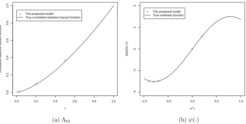
2.1 Spline functions . . . 26 2.2 Cumulative baseline hazard function Λ01 and nonlinear smooth

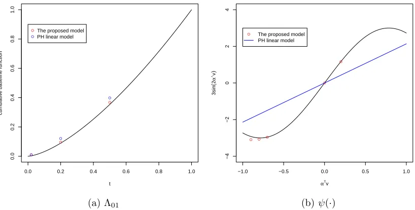
func-tion ψ(_∙) with their estimates at the chosen points. . . 37 2.3 Compare the proposed model and the PH linear model on cumulative

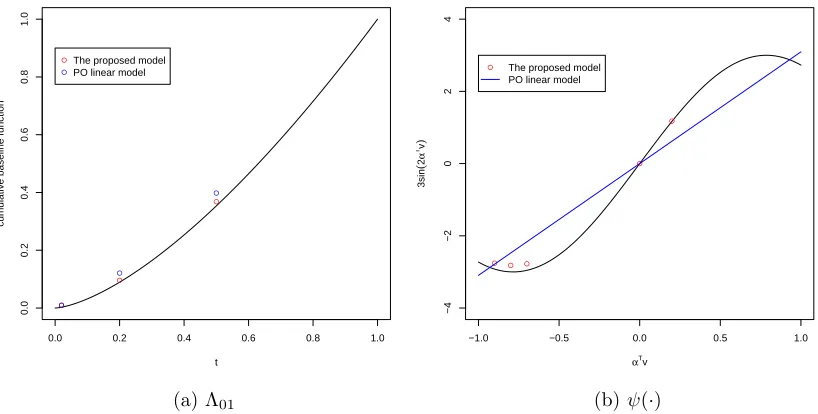
baseline hazard function Λ01 and nonlinear smooth function ψ(∙). . . 39

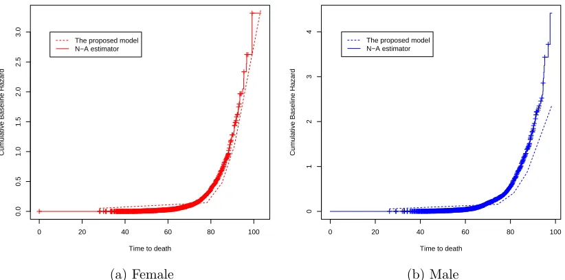
2.4 Compare the cumulative baseline hazard function Λ0 with N-A

esti-mator for female and male. . . 45 2.5 Compare the cumulative hazard function Λ considering covariate

ef-fects with N-A estimator of Λ0 for female and male. . . 45

2.6 Nonlinear function ψ(_∙) for females . . . 46 2.7 Nonlinear function ψ(∙) as the covariate age changes . . . 47 2.8 Nonlinear function ψ(_∙) as the covariate body mass index changes . . 47 2.9 Nonlinear function ψ(_∙) as the covariate cholesterol level changes . . . 48 3.1 Cumulative baseline hazard function Λ01 and nonlinear smooth

func-tion ψ(_∙) with the estimates at the chosen points. . . 60 3.2 Compare the proposed model and PO linear model on cumulative

base-line hazard function Λ01 and nonlinear smooth function ψ(∙). . . 63

3.3 Compare the cumulative baseline hazard function Λ0 of the proposed

model with N-A estimator for female and male . . . 67 3.4 Compare the cumulative hazard function Λ considering covariate

ef-fects with N-A estimator of Λ0 for female and male. . . 67

3.5 Nonlinear function ψ(_∙) for female . . . 69 3.6 Nonlinear function ψ(∙) as the covariate age changes . . . 69 3.7 Nonlinear function ψ(_∙) as the covariate body mass index changes . . 70 3.8 Nonlinear function ψ(_∙) as the covariate cholesterol level changes . . . 70 4.1 Nonlinear smooth function ψ(∙). . . 86 4.2 Compare the proposed transformation model and the transformation

linear model on the nonlinear smooth function ψ(∙). . . 89 4.3 The log likelihood profile of r . . . 92

(11)

1.1 Example data set . . . 4

2.1 The estimates for the covariate coefficients before and after transfor-mation . . . 35 2.2 The estimates for Λ01(∙) and ψ(∙) of one variate based on 200 runs . . 36

2.3 The estimates comparison of two models for the covariate coefficients α, β and φ based on 200 runs . . . 38 2.4 The estimates comparison of two models for Λ01(∙) and ψ(∙) based on

200 runs . . . 38 2.5 Simulation result for Weibull with shape parameter p= 0.5 of 200 runs 41 2.6 Simulation result for Weibull with shape parameter p= 1.5 of 200 runs 42 2.7 The estimates for the covariate coefficients α, β and φ of the data

analysis . . . 44

3.1 The estimates for the covariate coefficients before and after transfor-mation . . . 59 3.2 The estimates for Λ01(∙) and ψ(∙) of one variate based on 200 runs . . 60

3.3 The estimates comparison of two models for the covariate coefficients α, β and φ based on 200 runs . . . 62 3.4 The estimates comparison of two models for Λ01(∙) and ψ(∙) based on

200 runs . . . 62 3.5 Simulation result for Weibull with shape parameter p= 1.5 of 200 runs 65 3.6 The estimates for the covariate coefficients α, β and φ of the data

analysis . . . 66

4.1 The estimates for the covariate coefficients before and after transfor-mation (r= 1) . . . 85 4.2 The estimates for the covariate coefficients before and after

transfor-mation (r= 2) . . . 85 4.3 The estimates for ψ(_∙) of one variate based on 200 runs (r = 1) . . . . 86 4.4 The estimates for ψ(∙) of one variate based on 200 runs (r = 2) . . . . 86 4.5 The estimates comparison of two models for α, β, φ and r based on

200 runs (r= 1) . . . 88 4.6 The estimates comparison of two models for α, β, φ and r based on

200 runs (r= 2) . . . 88 4.7 The estimates comparison of two models for ψ(_∙) based on 200 runs

(12)

4.8 The estimates comparison of two models for ψ(_∙) based on 200 runs (r= 2) . . . 89 4.9 Simulation result for different settings of censoring rate, sample size,

association parameter φ . . . 90 4.10 Simulation result for different r . . . 92 4.11 Simulation result for assessing the proposed transformation model on

the generated data from nonlinear PH or PO model . . . 94

(13)

Introduction

Multivariate survival data arise frequently in health and medical studies. Examples

include epidemiological cohort studies, in which members from the same family can

have the same disease, and the ages at disease occurrence are collected; and clinical

trials, in which multiple event times are recorded for each individual. A common

characteristic of these data is that the survival times are correlated and it is not

appropriate to model them as independent events. To extract the scientifically

use-ful information from such data, it is appropriate to use multivariate, rather than

univariate, survival analysis techniques. On many occasions, the collected survival

times arise together with some other health related information, such as the gender,

age, smoking status etc., which are called covariates. One important motivation of

multivariate survival analysis is to investigate the covariate effects on the survival

times.

A variety of survival regression models have been developed over time to study

the covariate effects. A large body of literature exists for univariate survival data,

while the amount of work on the multivariate case is relatively smaller. The existing

multivariate regression models often assume linear relationships when exploring

co-variate effects. But the linearity assumption may be violated in many circumstances.

(14)

Chapter 1 2

We work to loosen this assumption and apply weakly parametric methods in

mul-tivariate regression models to explore nonlinear covariate relationships and to allow

more flexibility to the modeling.

In Section 1.1, real data examples are introduced to motivate the problems of

interest considered in this thesis. In Section 1.2, background literature and related

work are reviewed.

1.1 Motivation and Problem Description

Approaches used with multiple survival data vary according to different settings. If

the survival times are observed in some specified order, it is referred to as the longi-tudinal or sequential setting. If the multiple survival times have no prior ordering, it is called the parallel setting. In this thesis, we focus on the parallel setting. In the following two sections, examples of sequential data and parallel data are

intro-duced. In Section 1.1.3, the problems of interest, that will be studied in this thesis,

are summarized.

1.1.1 Colon Cancer Data

Moertel et al. (1990) conducted a clinical trial on patients with Duke’s stage C

colon cancer, a cancer stage at which disease recurrence is common after treatment.

The trial evaluated the efficacy of two treatments (a particular drug therapy and a

placebo). Two times were measured for each patient: time to cancer recurrence and

time from cancer recurrence to death. Because the two times are ordered—recurrence

must occur before death—this is an example of sequential data. Also, association can

be expected between the two responses, since each pair of times is measured on the

(15)

1.1.2 Busselton Health Study Data

The Busselton Health Study (Knuiman et al., 1994) was a repeated cross-sectional

survey that was conducted in the Busselton community in West Australia. From

1966 to 1981 a survey was conducted on adults in the community every three years.

Various health-related information was collected, such as demographic variables,

gen-eral health and lifestyle variables, health history variables, and physical, biochemical,

haematological and immunological measurements.

This data set includes the health information from 2306 couples who are adults

over 18 years old. The survival experience of the individuals, with survival time

defined as age at death, is considered here. This is an example of parallel multivariate

survival data, as the survival times of the husband and wife are likely to be associated

(because of their similar lifestyles), and there is no prior ordering associated with the

times. The censoring rate for female is 80%, and 67% for male. Excluding the censored

data, the average survival times for female and male are 75.2 and 74.2 respectively.

The data set has over ten health-related covariates, such as age at the beginning of

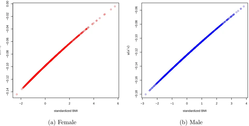
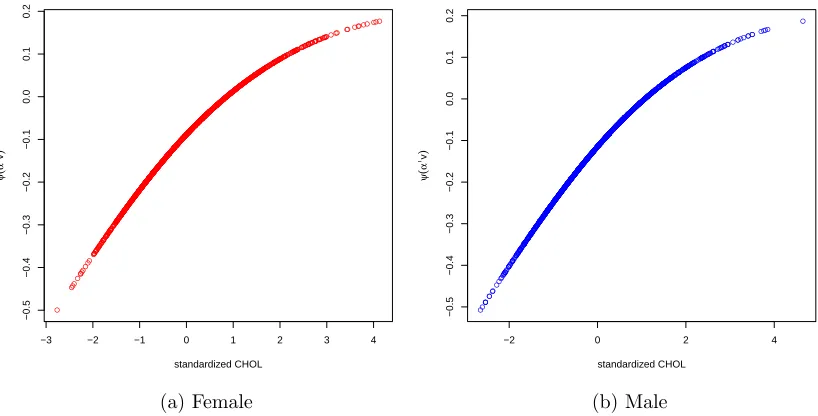
survey (AGE), body mass index (BMI), total cholesterol (CHOL), alcohol

consump-tion level (DRINKING), smoking status (SMOKE), and history of coronary heart

disease (CHD). A very brief look at a portion of the data set is found in Table 1.1.

The survival time is variable SURVTIME, and the censoring is recorded using the

death indicator DTHCENS.

1.1.3 Problem Description

Parallel multivariate survival data can be roughly classified into two groups. The

data can arise from different individuals. For example in the Busselton Health Study

data, the survival times of two members of a married couple tend to be associated, as

one family likely shares a similar diet and lifestyle. Alternatively, correlated data may

(16)

Chapter 1 4

Table 1.1: Example data set

No. PAIR SEX SURVTIME DTHCENS AGE BMI CHOL SMOKE ...

1 1 F 76.3 1 50.4 24.61 6.32 1 ...

2 1 M 80.4 0 52.3 27.37 6.13 1 ...

3 2 F 65.4 0 40.3 26.39 5.13 0 ...

4 2 M 65.6 0 40.5 29.54 5.79 1 ...

5 3 F 79.9 1 56.5 39.66 6.92 0 ...

6 3 M 78.5 1 66.8 23.63 7.11 1 ...

... ...

have different event timesTi1, . . . , Tik corresponding to different diseases. These times

can be associated, as they are influenced by the person’s health characteristics. Both

groups of data can be viewed as the same type of multivariate data. The subjects

that are correlated with each other, such as the people from the same family and

the diseases from the same individual, can be viewed as one cluster. Both types of parallel data can be dealt with using similar statistical approaches.

In most studies, survival data are collected along with some covariates.

Re-searchers are interested in finding the effects of the covariates on the survival time.

Another statistical question of interest is how to include the association of the data

in the modeling. In addition, being able to calculate the estimated survival function

or hazard function, after including the covariate effect in the model, is often required

in research. Regression models can be applied to solve these problems.

Many researchers have worked with various regression models for univariate

sur-vival data. Two regression models have drawn a lot of attention. One is the

pro-portional hazards (PH) model, and the other is the propro-portional odds (PO) model.

LettingT be the survival time and x= (x1, . . . , xp)T be the covariate, a PH model is

written as:

λ(t_|x) =λ0(t)exp(βTx),

(17)

of unknown parameters, and λ0(t) is the baseline hazard function when x=0 (Cox,

1972). PH models assume the covariates have a linear effect on the log hazards ratio.

This assumption is mainly for mathematical convenience, and it may be violated in

many situations. Such a linear structure also appears in the PO model. PO models

assume that the covariates have a linear effect on the log survival odds ratio:

S(t_|x)

1−S(t|x) = exp{β

T

x_} S0(t) 1−S0(t)

,

whereS(t_|x) is the survival function given the effects of covariate x,βis the covariate coefficient with dimension p×1, and S0 is the baseline survival function when x=0

(Bennett, 1983).

Various ways have been explored to loosen the linearity assumption. One approach

is to assume the covariate effect can be described by a flexible smooth function, rather

than a rigid log linear relation. To fit the smooth function, nonparametric methods

can be applied. In the application of the nonparametric methods there is one problem

that often occurs: the so-called curse of dimensionality. This term describes the phenomenon where the volume of the covariate space becomes too large to sample

thoroughly with any practical number of observations. In this case, the accuracy of

the estimation is often poor. To solve such a problem, a single index model may be

used to reduce the dimensions of the covariates. Hardle et al. (1993) generalize the

linear covariate effect βT

x intoψ(βT

x), where ψ is an unknown univariate function. This is called a single-index model. The single-index model uses the structure βT

x as the input of a smooth function, to reduce the high-dimensional variable x into a scalar, and the curse of dimensionality problem can be avoided.

In this thesis, the above ideas are applied to the modeling of multivariate survival

data. Three survival regression models are proposed and explored: the PH model, the

(18)

Chapter 1 6

covariate effects are added in the model by a smooth single index function, to loosen

the linearity assumption while reducing the high dimensions of the nonlinear covariate.

Spline functions are used to construct the nonlinear smooth function. Piecewise

constants are applied to model the baseline hazard function.

1.2 Literature Review

This section reviews regression methods for modeling multivariate survival data.

First, methods for incorporating the association among multivariate survival

re-sponses are introduced. Then a literature review on survival regression models is

given. Extensions on regression models, such as nonparametric approaches, are

sum-marized at the end.

1.2.1 Modeling Association in Multivariate Survival Data

One important question in multivariate survival data modeling is how to incorporate

the association. The common approaches may be distinguished as: marginal models,

frailty models and copula models.

The marginal model approach makes inferences about the marginal distributions

while treating the dependence among the subjects within one cluster as unspecified.

Indeed, it takes into account the dependence only while looking at the variance

esti-mates of the parameters. Therefore, parameters can be estimated from the marginal

model using the likelihood by assuming independence among all subjects, which is

the product of all the marginal likelihoods over all subjects. This likelihood is called

the Independence Working Model (IWM) (Huster et al., 1989).

There are two main issues arising from the IWM. One problem is the consistency

of the parameter estimates. It can be demonstrated that under certain conditions

(19)

consistent estimate in spite of the fact that observations are correlated. The other

one is for the appropriate variance estimators of parameters. The variance-covariance

structure of the data needs to be taken into account to arrive at good estimators for

the variances of the estimated parameters.

Cox proportional hazards model have been considered in the marginal model

ap-proach by many researchers. Wei, Lin, and Weissfeld (1989) and Lee, Wei, and Amato

(1992) have done such related work. The former allows the baseline hazard functions

to be different among the marginal models while the latter assumes a common

base-line hazard function. Lin (1994) summarizes and continues the work of both of the

previous two methods, and develops simple estimating equations which yield

con-sistent and asymptotically normally distributed estimators. The work also includes

robust variance-covariance estimators to account for the intra-class correlation. In

recent years, nonparametric methods have been explored in the marginal model. Yu

and Lin (2008) use kernel estimating equations to estimate nonparametric covariate

effects. They show the nonparametric kernel estimator is consistent for any arbitrary

working correlation matrix and its asymptotic variance is minimized by assuming

working independence.

The second approach to multivariate modeling is frailty models. Frailty models

are random effect models, which account for heterogeneity caused by unmeasured

covariates. The term frailty is introduced by Vaupel et al. (1979) in univariate survival

models and the model is substantially promoted by its application to multivariate

survival data by Clayton (1978) in a study of chronic disease incidence in families.

Hougaard (2000) provides broad discussions on this topic. Following the definition

from Lawless (2003), the common approach in frailty models is to define a random

(20)

Chapter 1 8

covariatexi, the survival timesTi1, . . . ,Tikare independent, with the survival function

Sij(tj) = Pr(Tij ≥tj|xi,αi) j = 1, . . . , k;

and (2) the αi are independent and identically distributed across all subjects i =

1, . . . , n. Assuming αi has distribution function G(αi;φ), the joint survival function

for Ti1, . . . , Tik is

S(t1, . . . , tk|xi) =

Z "_Yk

j=1

Pr(Tij ≥tj|xi,αi) #

dG(αi;φ),

where φ measures the dependence within the cluster. A common choice of the dis-tribution of αi is the gamma distribution. More general choices for this distribution

are discussed by Hougaard (2000).

Another approach to multivariate modeling is copula models. For simplicity, the

bivariate case is used as an example. A copula function is defined as a bivariate

function C: [0,1]2 _→_[0_,_{1], which satisfies the following three properties (Shemyakin}

and Youn, 2006):

1. C(u,0) = C(0, u) = 0 for any u_∈[0,1]. 2. C(u,1) = C(1, u) =u for any u∈[0,1]. 3. For all 0 ≤u1 ≤u2 ≤1 and 0 ≤v1 ≤v2 ≤1,

C([u1, v1]×[u2, v2]) =C(u2, v2)−C(u1, v2)−C(u2, v1) +C(u1, v1)≥0.

Therefore, when the arguments of the copula function are univariate survival functions

S1(t1) = P(T1 > t1) and S2(t2) = P(T2 > t2), the copula function C(S1, S2) is a

bivariate survival function S(t1, t2) = P(T1 > t1, T2 > t2), with marginal survival

(21)

Development of the joint survival function can be done through the specification

of a parametric copula function C(u, v;φ) and the specification of the marginal distri-butions. Parameter φdetermines the association structure of the data. The marginal survival functions S1(t1) and S2(t2) can have parametric or semiparametric forms.

One such family of copula models is introduced by Clayton (1978). It has the

form

S(t1, t2) =

h

S1(t1)−φ

−1

+S2(t2)−φ

−1

−1i−φ. (1.1) whereφ ∈(0,∞). The larger the value of φis, the smaller the association among the data is. When φ =_∞, the two survival times are independent. The range of φ can be extended to -1 to accommodate some negative association (Lawless, 2003).

Note that for copula models the parameter φ only controls the association but does not enter into the marginal distributions, while in frailty models φ not only controls the association, but also affects the marginal distributions. A frailty model

is more appropriate for designed studies where different treatments or covariate factor

levels are assigned to individuals within a cluster.

1.2.2 Univariate Regression Models for Survival Data

The widely used survival regression models are the proportional hazards (PH) model,

the accelerated failure time (AFT) model, and the proportional odds (PO) model.

In recent years, the linear transformation model has also drawn many researchers’

attention. We will discuss each of these models in turn.

Cox (1972) proposes the Cox proportional hazards function with the following

form:

λ(t|x) =λ0(t)exp(βTx), (1.2)

where λ0(t) is the baseline hazard function, x = (x1, x2, . . . , xp)T is the vector of

(22)

Chapter 1 10

vector of regression coefficients. The model makes no assumptions on the baseline

hazard function λ0(t), but assumes a parametric form for the effect of the predictors

on the hazard. Therefore, it is referred to as a semi-parametric model. To make

inference, the partial likelihood approach (Cox, 1975) can be applied. The beauty of

this model is that the vagueness of the baseline hazard function creates no problem

for estimation.

Note that covariates act multiplicatively on the hazard function in the Cox PH

model. One assumption of the Cox model is that the hazard of the event in one

group is proportional to the hazard in any other. To apply this model properly the

proportionality assumption needs to be satisfied.

The PH model can be generalized to have the form

λ(t|x) =λ0(t)r(ψ(x)),

where r(_∙) is a positive function, and ψ(x) is usually assumed to be of linear regres-sion form ψ(x) = βT

x. Conventionally, r(_∙) = exp(_∙) can be applied to satisfy the positivity constraint. When λ0(t) is unspecified, it is referred to as the Cox model.

When λ0(t) is assumed to follow a specific distribution, it is called a parametric PH

model. More generally, λ0(t) can be specified as a piecewise constants or a spline

function (He and Lawless, 2003), in which case the full likelihood approach can be

applied.

Another popular model for survival data is the Accelerated Failure Time (AFT)

model. The AFT model usually can be written as a log-linear model for failure time

T according to:

logT =μ+α1x1+α2x2+∙ ∙ ∙+αpxp+σ.

(23)

the survival function of :

S(t) = P(T _≥t) = P (logT _≥logt)

= P (μ+α1x1+α2x2+∙ ∙ ∙+αpxp +σ≥logt)

= P

_≥ logt−μ−α

T_x

σ

= S

logt−μ−αT_x

σ

Another way of expressing the AFT model is

S(t_|x) =S0(η(x)t),

whereS0(∙) is the baseline survival function, andη(∙) is an “acceleration factor” which

depends on the covariates x= (x1, x2, . . . , xp)T through the formula:

η(x) = exp(α1x1 +α2x2 +∙ ∙ ∙+αpxp).

In this model the effect of a covariate is to stretch or shrink the survival curve along

the time axis by a constant relative amount η(x).

In AFT models, it is often necessary to specify the distribution of failure time.

The common distributions used for this purpose are Weibull, Log-normal, Log-logistic,

and Gamma. Some other approaches have also been discussed by researchers. Wei

(1992) reviews some estimation methods applied to the AFT model. For example,

an estimation procedure based on rank test statistics, and an approach using least

squares principle proposed by Buckley and James (1979) are discussed. Recently, Jin,

Lin, Wei, and Ying (2003) and Jin, Lin, and Ying (2006) develop approximations to

(24)

Chapter 1 12

Resampling procedures are applied for the estimation of the limiting covariance

ma-trix.

A third popular approach for survival data modeling is the Proportional Odds

(PO) model, which is introduced by Bennett (1983). This model uses the survival

odds ratio as a measure of relative risk in the regression model. It can be expressed

as:

S(t|x)

1₋S(t_|x) = exp(β

T

x) S0(t) 1₋S0(t)

, (1.3)

where x = (x1, x2, . . . , xp)T is the vector of explanatory variables for an individual,

β = (β1, β2, . . . , βp)T is the vector of regression coefficients, and S0(t), the baseline

survival function, is the survival function for an individual whose explanatory

vari-ables all take the value zero.

One important property of PO model is that the hazards ratio converges from the

value exp(−βT

x) at time t = 0, to unity at t = ∞. It can be shown that (Collett, 2003)

λ(t|x)

λ0(t)

= [1 + (exp(βT

x)−1)S0(t)]−1.

Therefore, when t = 0, S0(t) = 1, and λ_λ(t₀|x₍_t₎) = exp(−βTx); when t =∞, S0(t) = 0,

and λ_λ(t|x)

0(t) = 1. As a contrast, in the PH model, the hazards ratio remains constant

att. Recall that for the PH model,

λ(t|x)

λ0(t)

= exp(βT

x),

but this assumption can be unreasonable in certain circumstances. For example,

initial effects such as differences in the stage of disease or in treatment can disappear

with time. In this case, the property of PO model that the hazards ratio converges

to 1 as t increases to _∞makes more sense.

Bennett (1983) describes how the PO model can be fitted using maximum

(25)

properties of the PO model. Many researchers have discussed various approaches for

making inferences on PO model. Cheng et al. (1995) propose a modified V statistic for parameter estimation. Murphy et al. (1997) show the profile likelihood approach

of Bennett (1983) results in an asymptotically efficient regression estimator. Yang and

Prentice (1999) introduce some weighted empirical odds functions. Several classes of

regression estimators such as the psedo-maximum likelihood estimator, martingale

residual-based estimators, and minimum distance estimators are derived.

The final model considered here is the linear transformation model. Let T be the survival time andxbe the covariate with dimension p_×1. The linear transformation model assumes that

H(T) = ₋βT

x+, (1.4)

where H is an increasing transformation function, is a random variable with a known distribution, and β is the covariate coefficient with dimension p×1. The proportional hazards model and the proportional odds model are special cases of (1.4)

withfollowing the extreme-value distribution and the standard logistic distribution, respectively.

An alternative way to show that the PH and PO models are the special cases of

the transformation model is though the hazard function of . If we let the hazard function of have the form

λ() = exp() 1 +rexp(),

then r= 0 corresponds to a PH model, and r= 1 corresponds to a PO model. More discussion related to this topic is given in Section 4.1.

Some inference procedures for this model have been proposed by various

re-searchers. Cheng et al. (1995) study a class of generalised estimating equations to

examine the covariate effects with censored observations. This method is further

(26)

Chapter 1 14

assumption in their approach is that the censoring variable is independent of the

covariates, which makes it possible to use the Kaplan-Meier method to estimate the

survival function. Chen et al. (2002) relax this assumption and propose an estimating

equation approach to make inference. Zeng and Lin (2006) study nonparametric

max-imum likelihood estimation in a class of semiparametric transformation models which

considers time dependent covariates. More recently, Lu and Zhang (2010) propose

a partially linear transformation model by incorporating nonlinear covariate effects,

and studied a martingale-based estimating equation approach to make inference.

1.2.3 Extensions on Regression Models

A lot of work has been done on extensions of regression models. As mentioned

pre-viously, one of the traditional assumptions of regression models is that the covariates

have a linear effect on the log hazards ratio, log survival odds ratio, or other quantity

of interest. However, this linearity assumption is mainly for mathematical

conve-nience, and might not be valid in many circumstances. A smooth function ψ(_∙) has been proposed to generalize the linearity assumption βT

x. In the exploration of the smooth function, nonparametric or the weakly parametric methods have drawn much

attention. Tibshirani and Hastie (1987) use the linear regression method on a defined

local neighborhood of each x. This local likelihood estimation approach is applied to find the optimal estimator of the local regression coefficients. Note that this local

linear regression model can also be replaced by some other smooth function. Fan,

Gijbels, and King (1997) discuss the estimation of the nonparametric covaritate effect

in the PH model when the baseline function is parametric and nonparametric. When

the baseline function and the covariate effect are both unspecified, nonuniform kernel

methods are applied to fit the covariate effect and the inference is based on a local

version of partial likelihood. Spline functions have also been considered by some

(27)

nonparametric covariate effect in PH models. An automatic procedure involving the

maximum likelihood method, stepwise addition, stepwise deletion and BIC is used to

select the final model.

A considerable amount of work has been done to address the curse of

dimensional-ity problem under the univariate data modeling framework when the covariates have

high dimension. One approach is to use additive models. Hastie and Tibshirani (1990)

propose to use a sum of smooth functions over the components of covariates. That

is, instead of using the linear model Pp_j₌₁xijβj, they suggest using an additive term Pp

j=1fj(xij), where xi1, . . . , xip are covariate values for the ith individual. The fj(∙)

are unspecified smooth functions that are estimated using scatter plot smoothers.

The other approach that has drawn a lot of attention is the single index model.

Har-dle et al. (1993) generalize the linear covariate effect βT

x intoψ(βT

x), where x is a

p×1 vector of covariates, β is a p×1 vector of parameters, and ψ is an unknown univariate function. This single index model reduces the p×1 vector of covariates x from higher dimensions to a scalar βT

x, and then treats the smooth function ψ(∙) as a univariate function of βT

x. Note the scale of βT

x in ψ(βT

x) may be determined arbitrarily, soβ may be replaced by the unit vector α=β_kβ_k−1_{, where}_{k ∙ k}_denotes

the Euclidean metric. Then we can estimate both ψ(_∙) and α in the model.

Because of the useful characteristic of the single index model that it can reduce the

the high dimension of covariates to a scalar, it has drawn a lot of attention from many

researchers. Carroll, Fan, Gijbels, and Wand (1997) apply it to the generalized linear

model and introduces a more general model which is called “Generalized Partially

Linear Single Index Model (GPLSIM)”. In this model a response Y is to be predicted by covariates (X,V), where X (of length p) is to enter the model linearly and V (of length q) is to enter it nonlinearly. GPLSIM has the following form:

g{μ(x,v)}=βT

x+ψ(αT

(28)

Chapter 1 16

whereμ(x,v) = E(Y),g is the link function, ψ is an unknown smooth function, and αand β are coefficients of dimensions q and p. The single index structure ψ(αT_{v) is}

added to extend the linear termβT

xwhich the generalized linear model normally has, and makes it more flexible to describe a nonlinear relationship between the covariate

(x,v) and g{μ(x,v)}. Kernel methods are used to explore the shape of the smooth function ψ nonparametrically.

In recent years, structures similar to GPLSIM have been applied in some

sur-vival models. For example, Lu, Chen, Singh, and Song (2006) introduce the partially

linear single index structure under the proportional hazards regression model

frame-work, and define a “Partially Linear Single-Index Survival Model (PLSISM)”. More

information about this model can be seen in Section 2.1.

The above work mainly focuses on the extensions of regression models for

univari-ate survival data. There is still limited work for regression modeling of multivariunivari-ate

survival data, however, especially on the exploration of nonparametric methods

ap-plied in regression models. He and Lawless (2003) use piecewise constant or spline

functions to fit the baseline hazard function in either marginal or conditional

propor-tional hazards models. The copula model is proposed to incorporate the association

among the multivariate survival data. As the baseline hazard function has a specified

form through the parametric approach, full likelihood can be applied to make

infer-ence. Yu and Lin (2008) study multivariate survival data through the marginal model

approach. They propose the marginal proportional hazards function and use kernel

methods in the regression model. They show that the nonparametric kernel estimator

is consistent for any arbitrary working correlation matrix and its asymptotic variance

is minimized by assuming working independence. These works have given inspiring

(29)

1.3 Overview of the Thesis

The focus of this thesis is on multivariate survival data regression modeling.

Cop-ula functions are proposed to include the association among the multivariate

sur-vival data, with covariate effects incorporated through the marginal model. For the

marginal distributions, three types of regression models are discussed: (i) the

pro-portional hazards function, (ii) the propro-portional odds model, (iii) the generalized

transformation model. Traditionally, these models assume the covariates have linear

effects in the regression part of the model. We relax the linearity assumption and

allow both the linear and the nonlinear relationships in the model. A smooth

func-tion is used to explore the nonlinear relafunc-tionship. The single index model is added to

reduce the dimensions of the nonlinear covariates into a scalar. Weakly parametric

methods are applied to explore the smooth function. In the marginal hazard

func-tion, piecewise constants are used to estimate the baseline hazard function. Based

on the above setup of the model, the full likelihood function can be applied to make

inference.

The remaining chapters of the thesis are organized as follows. In Chapter 2 the

partially linear single index proportional hazards regression model for multivariate

survival data is investigated. The proposed model is assessed by simulation studies.

The model is applied to the real data example, Busselton Health Study, for

illustra-tion. In Chapter 3 the partially linear single index proportional odds regression model

is explored. Simulation studies and real data analysis are also provided. Chapter 4

examines the partially linear single index generalized transformation model. As the

PH model and the PO model are two special cases of the generalized transformation

model, the third proposed model is a generalization of the first two. Simulation

stud-ies are provided. Some conclusions are discussed at the end of Chapter 4. Discussions

(30)

Chapter 2 Flexible Partially Linear Single

Index Proportional Hazard

Regression Model for Multivariate

Survival Data

2.1 Introduction

The proportional hazards model (1.2) has been a very popular survival model since

it was proposed by Cox (1972). One of the assumptions of the PH model is that the

covariatexhas a linear effect on the log hazards ratio. This assumption is mainly for mathematical convenience, however, may not hold in many situations. Many methods

have been proposed to add a smooth function ψ(_∙) to relax the linearity assumption, letting the covariate effect be written as βT

x+ψ(v). In this expression x is a vector of covariates that enter the model linearly, and v is a vector of covariates that enter in a nonlinear fashion. This is called a partially linear model.

(31)

drawn much attention. However, if vis high-dimensional covariate vector, the curse of dimensionality problem (described in Section 1.1.3) makes it hard to achieve accurate

estimation for covariate effect ψ(v) using nonparametric methods.

One approach to solve this issue is through the use of single index models (Hardle

et al., 1993). In this approach, a new parameter vector α is introduced, and the inner product αT_v _{is taken to reduce the covariate effects to a scalar, to summarize}

covariates first. The smooth function ψ(∙) is then taken to be a function of this scalar argument. This particular type of partially linear model, with the covariate effect

taking the form βT

x+ψ(αT_{v), is known as a partially linear single index model.}

Partially linear single index models have been explored in the literature. For

example, Lu, Chen, Singh, and Song (2006) propose the Partially Linear Single-Index

Survival Model (PLSISM). The hazard function has the form:

λ(t|x,v) = λ0(t)exp{βTx+ψ(αTv)}, with kαk= 1,

where λ0(t) is the baseline hazard function, ψ(∙) is the unknown smooth function, x

is the linear covariate with dimension p, v is the nonlinear covariate with dimension

q, and β and αare their corresponding coefficients. The authors use kernel methods to model the smooth function. The profile quasi-likelihood approach is applied to

make inference. Sun, Kopciuk, and Lu (2008) also apply a similar partially single

index structure in proportional hazards regression. They use spline functions to

approximate the smooth function. In their model, the baseline hazard function is not

specified, and the partial likelihood approach is applied for inference.

The above work has been done under the univariate response framework. We

propose to apply the partially linear single index structure in the marginal hazard

function for multivariate data. As has been introduced in Section 1.2.1, a copula

(32)

Chapter 2 20

data. Without loss of generality, a special case of multivariate data–bivariate data–is

considered here. Specifically, the Clayton model (Clayton, 1978) is employed to link

the marginal survival functions for illustration.

To make inference, two parts of the model still need to be specified. One is the

baseline hazard function, and the other one is the smooth function in the single

index structure. The objective we consider here is to model these functions without

making overly strong parametric assumptions, while also choosing a form that is

flexible enough. To do this, two weakly parametric approaches, piecewise constants

(He and Lawless, 2003) and spline functions, are proposed to model the baseline

hazard functions and the smooth function respectively. This model structure has

finite number of parameters, and therefore the full likelihood method can be invoked

for inference.

The details of the proposed model framework is introduced in Section 2.2.

Simu-lation studies are conducted in Section 2.3, to assess the performance of the proposed

method, to compare the proposed model to the model where the nonlinear covariate

effect is ignored, and to evaluate the impact of other factors on the estimation

un-der various scenarios. The Busselton health study is used as an illustrative example.

Some conclusions about the proposed model are summarized at the end.

2.2 The Proposed Model

Assume the survival data sample has m clusters. Let Tij and Cij be the failure and

censoring times of the jth observation in the ith cluster (j = 1, . . . , k, i= 1, . . . , m). The observed data (yij,xij,vij, δij) are realizations of the variables (Yij,Xij,Vij,Δij),

where Yij = min(Tij, Cij) is the observed time, and Δij =I(Tij ≤ Cij) is the

censor-ing indicator. The covariates are Xij andVij, which are assumed to have linear and

(33)

correlated, while the observations from different clusters are assumed to be

indepen-dent. For illustration purpose, we assume k = 2, to limit the survival distribution to be bivariate. The proposed marginal PH function is written as:

λj(tj|xj,vj) =λ0j(tj)exp{βTxj +ψ(αTvj)}, j = 1, 2,

where β is the linear covariate coefficient with dimension p and α is the nonlinear covariate coefficient with dimension q,ψ(_∙) is a smooth function, and ψ(αT_v

j) is the

single index model.

To incorporate the association in the model, a copula model is used for multivariate

modeling (see Section 1.2.1). More specifically, the Clayton model (Clayton, 1978) is

used, and the joint survival function is given by (1.1).

Let f(t1, t2) denote the joint density function. The likelihood contributed from

the ith cluster is,

Li = f(ti1, ti2)δi1δi2

"

−∂S(ti1, ti2)

∂ti1

#δi1(1−δi2)

×

"

−∂S(ti1, ti2)

∂ti2

#(1−δi1)δi2

S(ti1, ti2)(1−δi1)(1−δi2), (2.1)

which is also shown in Lawless (2003).

To make inference from the model, we need to write this likelihood explicitly as

a function of the parameters. To do this, the estimation approaches for the baseline

hazard functions λ0j(tj) and the smooth function ψ(∙) need to be specified. We

propose to use piecewise constant approach (He and Lawless, 2003) to approximate

the baseline hazard functions, and to use a spline function approach to approximate

(34)

Chapter 2 22

2.2.1 Piecewise Constant Approach for Baseline Function

In modelling the baseline hazard function λ0j(tj), we follow He and Lawless (2003),

to have a piecewise constant function approximation. Compared with the parametric

PH model, which assumes that the baseline hazard function has a known parametric

form, this method relaxes the parametric assumption of λ0j(tj) to allow flexibility in

its shape.

Assume that the marginal baseline hazard functions λ0j(tj), j = 1,2,have

piece-wise constant forms as follows:

λ01(t1) =ρk, wheret1 ∈Ak= (ak−1, ak], k= 1, . . . , r,

and

λ02(t2) =τl, where y2 ∈Bl= (bl−1, bl], l= 1, . . . , s,

where 0 = a0 < a1 < . . . < ar = ∞ and 0 = b0 < b1 < . . . < bs = ∞ are

pre-chosen sequences of constants, which are also called cut points. ρ= (ρ1, . . . , ρr)T and

τ = (τ1, . . . , τs)T are unknown positive constants to be estimated. Ak and Bl are the

intervals defined by the sequence of cut points. Therefore, the corresponding marginal

cumulative hazard functions are the integration over the piecewise constants, which

can be written as:

Λ01(t1) =

r X

k=1

ρkuk(t1)

Λ02(t2) =

s X

l=1

τlwl(t2),

where uk(t1) = max(0,min(ak, t1)−ak−1) are the length of the intersection of the

interval (0, t1) with the interval Ak, and wl(t2) = max(0,min(bl, t2)−bl−1) are the

(35)

How to choose the cut points is an important question. Normally they are chosen

based on prior assumptions about the marginal distributions of the survival time. If

we know the hazard function slope changes at some points, these points can be set as

the cut points. If such changes can not be detected clearly, one can start from a small

number of cut points, say 2 or 3, and increase the number to observe their effect.

Normally it is desirable to keep roughly the same number of failures within each

interval. For data with a high censoring rate, one useful way to choose the cut points

is based on the Kaplan-Meier survival probability without considering the covariate

effects. That is, use the cut points that give roughly the same survival probability

in each interval. In our simulation study and real data analysis, since the censoring

rate can be high, we use the strategy based on survival probability. We choose to use

four intervals (r = s = 4) to approximate the baseline hazard function, which can give reasonably good estimation (Lawless and Zhan, 1998), and keep the number of

parameters in the model to a manageable level.

2.2.2 Spline Function Approximation

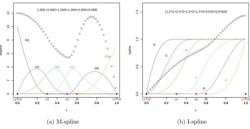
Spline methods are used to estimate the smooth functionψ(∙). M-spline functions and I-spline functions (Ramsay, 1988) are proposed to approximate ψ(∙), because of their convenient characteristics. By definition, M-spline basis functions are nonnegative

functions. I-spline basis functions are defined as the integration of the corresponding

M-spline basis functions, and have the property of being monotone increasing. In the

proposed model we would like to model the smooth function ψ(_∙) and its derivative

ψ0₍_∙_{). Therefore, it is very natural to use M-spline functions to approximate the} derivative ψ0(∙), and use I-spline functions to approximate the smooth function ψ(∙). Note that while the I-spline basis functions are monotone, the I-spline itself will not

be monotone unless the coefficients are restricted to be positive. In the proposed

(36)

Chapter 2 24

flexible shape.

A spline function is a series of polynomials joined smoothly at some break points.

Given an interval [L, U] and the breakpoints η =_{η0, . . . , ηk}, where L=η0 <∙ ∙ ∙<

ηk = U, there is one corresponding polynomial function Pj of order m or degree

m-1 on each subinterval [ηj, ηj+1) called a basis spline function. The spline function is

defined asf(x) =Pk_j₌₁cjPj(x), wherecj is the corresponding coefficient for each basis

spline function. At the boundaries of the intervals, a certain degree of smoothness

is required. The smoothness is defined by the equality of the derivatives of Pj. A

popular choice is to let the derivatives be continuous up to order two at the break

points, as our human eyes are capable to detect the discontinuity no higher than the

second order.

The M-spline and I-spline functions are both defined based on a sequence of

“knots”. Once the breakpoints for the interval [L, U] are given, η = {η0, . . . , ηk},

the sequence of knots c={c1, . . . , ck+2m−1}are constructed as

c1 =. . .=cm =η0, ck+m =. . .=ck+2m−1 =ηk,

and

cm+j =ηj, j = 1,2, . . . , k−1.

Let Mi(x|1, c) be the ith M-spline basis function of order m with knot sequence c.

These basis functions are defined recursively:

Mi(x|1, c) =       

1

ci+1−ci if ci ≤x < ci+1,

(37)

and for m >1, :

Mi(x|m, t) =

m[(x−ci)Mi(x|m−1, c) + (ci+m−x)Mi+1(x|m−1, c)]

(m₋1)(ci+m−ci)

.

One main characteristic of M-spline function is that the basis spline functions

are positive within the interval (ci, ci+m) and zero otherwise. In total there are k+

m₋1 of them for spline function of order m. Figure (2.1a) gives one example of a group of cubic M-spline basis function on the interval of (0,1), and the breakpoints

(0.3,0.5,0.6). The basis spline functions are M1, M2, . . . , and M6. The function

f(x) = 1.2M1+ 2.0M2+ 1.2M3+ 1.2M4+ 3.0M5+ 0.0M6, is represented by the top

dotted line.

I-spline functions are defined based on the M-spline functions. The basis functions

are the integration of the corresponding M-spline basis functions:

Ii(x|m, c) = Z x

L

Mi(u|m, c)du.

The definition can be expressed in the following form:

Ii(x|m, c) =               

0 i > j,

Pj

n=i(cn+m+1−cn)Mn(x|m+ 1, c)/(m+ 1), j−m+ 1≤i≤j,

1 i < j₋m+ 1.

Figure (2.1b) shows the spline function corresponding to Figure (2.1a). The

I-spline basis functions I1, . . . , I6 are shown as dashed lines. They are the integrations

of the corresponding M-spline basis functions M1, . . . , M6. The I-spline function

g(x) = (1.2I1+ 2.0I2+ 1.2I3+ 1.2I4 + 3.0I5 + 0.0I6)/6, is represented by the dotted

line.

(38)

Chapter 2 26

● ● ● ●_● ●_●

● ●

●_{● ● ●}● ●

● ●

● ●●

● ● ● ●

● ●

●

0.0 0.2 0.4 0.6 0.8 1.0

0

2

4

6

8

10

12

x

Mspline

0.0 0.2 0.4 0.6 0.8 1.0

● ● ● ● ●

M1

M2 M3 M4 _M5 M6

1.2M1+2.0M2+1.2M3+1.2M4+3.0M5+0.0M6

c1−c3 c4 c5 c6 c7−c9

(a) M-spline

●● ●●

● ●●

●● ●●

●● ●●●

●●●● ●●

●● ●●

● ●● ●

0.0 0.2 0.4 0.6 0.8 1.0

0.0

0.5

1.0

1.5

x

Ispline

0.0 0.2 0.4 0.6 0.8 1.0

● ● ● ● ●

I1

I2

I3

I4

I5

I6

(1.2*I1+2.0*I2+1.2*I3+1.2*I4+3.0*I5+0.0*I6)/6

c1−c3 c4 c5 c6 c7−c9

(b) I-spline

Figure 2.1: Spline functions

Mj,j = 1, . . . , d, be the M-spline basis functions, and M(u) = (M1(u), . . . , Md(u))T.

Then ψ0_(αT_{v) can be written as:}

ψ0(αT_{v) =} d X

j=1

γjMj(αTv) =γTM(αTv),

where γj is the coefficient for the jth basis function.

By definition, I-spline functions can be used to fit ψ(∙), as the basis function is the integration of the corresponding M-spline basis function. Note that ψ(0) is constrained to be 0. This is because in the regression model βTx+ψ(αT_{v), we want}

the intercept to be 0, which implies βTx = 0 for x = 0 and ψ(0) = 0. Using this constraint, ψ(αT_{v) can be modeled by} RαTv

(39)

ψ(αT

v) =

Z αTv

0

ψ0(x)dx

=

Z αT_v

0

d X

j=1

γjMj(x)dx

=

d X

j=1

γj

Z αTv

0

Mj(x)dx

=

d X

j=1

γj

Z αT_v

L

Mj(x)dx− d X

j=1

γj Z 0

L

Mj(x)dx

=

d X

j=1

γj[Ij(αTv)−Ij(0)]

= γT_[_I_(αT_v)

−I(0)]

Note there are another two constraints in the marginal PH model, and both are

related to parameter identifiability. One constraint is, for ψ(αT_{v) we need}_k_α_k_{= 1.}

If the norm of α is not specified, the sets of solutions for α are not unique, and the solutions for γ are also not unique. But only with this one constraint, we are still not able to find the unique solution for γ and α. The other constraint is to let one particular component of α(for example, its last element) be positive. This is because

ψ∗₍₋_{α) =} _ψ_{(α), therefore for} _ψ∗_, ₋_α _{is the solution, and for} _ψ_, _α _{is the solution.} That is, both (α,γ) and (−α,−γ) are solutions for the smooth function. With these two additional constraints, it is possible to find unique solutions for γ and α.

Regarding the strategy of choosing the number of breakpoints, we follow the

advice given by Lawless and Zhan (1998), who suggest to use 4-10 intervals. In the

simulation study and the real data analysis, in order to satisfy the goal of having

good model performance and not too long of a simulation time, 4 intervals (i.e.,3

breakpoints) are chosen in spline functions. Each interval contains roughly the same

(40)

Chapter 2 28

2.2.3 The Likelihood

Now that the baseline hazard function λ0j(tj) and the smooth function ψ(∙) have

been fully specified, the likelihood as given in equation (2.1) can be worked out.

Using the relationship between the survival function and the hazard function, the

marginal survival functions can be written as shown below. Note that in the following

expressions we write Sij(tij) rather than Sij(tij|xij,vij) for notational simplicity. In

the remainder of the thesis we will use these two notations for the survival function

interchangeably.

Si1(ti1) = exp

h

−Λ01(ti1)exp{βTxi1+ψ(αTvi1)}

i

, Si2(ti2) = exp

h

−Λ02(ti2)exp{βTxi2+ψ(αTvi2)}

i

,

where Λ01(ti1) =Prk=1ρkuk(ti1), Λ02(ti2) = Prl=sτlwl(ti2), and

ψ(αT

vi1) = γT[I(αTvi1)−I(0)],

ψ(αT_v

i2) = γT[I(αTvi2)−I(0)].

Note, in the proposed model, the linear covariate coefficients and the nonlinear

co-variate coefficients are assumed to be same for the two members of the same cluster

(that is, coefficients β, α, and γ are the same for j = 1 and j = 2). The reason for this is to control the list of the parameters to a manageable level and to avoid long

run times in simulations. The natural extension is to assume the linear and nonlinear

covariate coefficients are different for the two variates. This extension poses no

diffi-culties if computation time is not a concern, as estimation and inference procedures

are unaffected.

(41)

given in Formula 1.1. The log likelihood is written as:

l =

n X

i=1

logLi

=

n X

i=1

(

δi1δi2logf(ti1, ti2)

+δi1(1−δi2)log

h

−∂S(ti1, ti2)

∂ti1

i

+(1−δi1)δi2log

h

−∂S(ti1, ti2)

∂ti2

i

+(1₋δi1)(1−δi2)logS(ti1, ti2)

)

(2.2)

The entries of the log likelihood function −∂S(ti1,ti2)

∂ti1 ,

−∂S(ti1,ti2)

∂ti2 , and f(ti1, ti2) are

given as follows:

−∂S(ti1, ti2)

∂ti1

= −

∂hSi1(ti1)−φ

−1

+Si2(ti2)−φ

−1

−1i−φ

∂ti1

= ₋hSi1(ti1)−φ

−1

+Si2(ti2)−φ

−1

−1i−φ−1hSi1(ti1)−φ

−1i

×exp_{βT

xi1+ψ(αTvi1)}

∂[₋Λ01(ti1)]

∂ti1

−∂S(ti1, ti2)

∂ti2

= −

∂hSi1(ti1)−φ

−1

+Si2(ti2)−φ

−1

−1i−φ

∂ti2

= ₋hSi1(ti1)−φ

−1

+Si2(ti2)−φ

−1

−1i−φ−1hSi2(ti2)−φ

−1i

×exp_{βT_x

i2+ψ(αTvi2)}

∂[₋Λ02(ti2)]

(42)

Chapter 2 30

f(ti1, ti2) =

∂S(ti1, ti2)

∂ti1∂ti2

= hSi1(ti1)−φ

−1ih

Si2(ti2)−φ

−1i

exp_{βT_x

i1 +ψ(αTvi1)}

×exp{βT

xi2+ψ(αTvi2)}

∂[−Λ01(ti1)]

∂ti1

×∂[−Λ02(ti2)]

∂ti2

h

Si1(ti1)−φ

−1

+Si2(ti2)−φ

−1

−1i−φ−2(1 +φ−1)

2.2.4 Parameter Estimates

The likelihood function involves the following parameters:

θ = (φ,ρT_,_τT_,_αT_,_βT

,γT₎T_,

where φ is the association parameter; ρ and τ are the parameters for the piecewise constants, and ρ = (ρ1, . . . , ρr)T, τ = (τ1, . . . , τs)T; α are the nonlinear covariate

parameters with α= (α1, . . . , αq)T; β are the linear covariate parameters with β =

(β1, . . . , βp)T; and γ are the parameters for spline functions with γ = (γ1, . . . , γd)T.

Recall, some of the parameters have constraints required by the model, which are

summarized as follows:

ρ1, . . . , ρr >0,

τ1, . . . , τs >0,

φ >0,

kα_k= 1, and αq >0,

ψ(0) = 0.

The question now is how to find the maximum likelihood estimates of the

param-eters, which actually becomes an optimization problem. The constraints will bring

(43)

the process of optimizing the solutions. To avoid such problem, we introduce some

new parameters which are transformed from the original parameters. Through the

transformation, the new parameters will have no constraints.

For positive parameters ρk, τl, and φ, a log transformation is applied. New

pa-rameters ξk,ζl and % are introduced as given below:

ξk = logρk, k = 1, . . . , r.

ζl= logτl, l = 1, . . . , s,

%= logφ.

For α, the transformation takes two steps. First we use the trigonometric trans-formation on αfor the constraint kαk= 1, and make sure the last component of α is positive. Parameter ω is introduced with ω= (ω1, . . . , ωq−1)T. That is:

α1 = sinω1sinω2∙ ∙ ∙sinωq−2sinωq−1

α2 = sinω1sinω2∙ ∙ ∙sinωq−2cosωq−1

. . . (2.3)

αq−1 = sinω1cosω2

αq = cosω1

where ω1, . . . , ωq−1 ∈[−π₂,π₂] and ω1 ∈[−π₂,π₂] can satisfy αq >0.

(44)

Chapter 2 32

new parameter ϕ is introduced, where ϕ = (ϕ1, . . . , ϕq−1)T:

ϕ1 = log

π

2 +ω1

π

2 −ω1

⇒ω1 =

eϕ1 −₁

eϕ1 + 1

π

2

ϕ2 = log

π

2 +ω2

π

2 −ω2

⇒ω2 =

eϕ2 −₁

eϕ2 + 1

π

2 (2.4)

. . . ϕq−1 = log

π

2 +ωq−1

π

2 −ωq−1

⇒ωq−1 =

eϕq−1 ₋₁

eϕq−1 + 1

π

2

Through the two steps of transformation the relationship between α and ϕ are as follows:

α1 = sin

h_eϕ1 ₋₁

eϕ1 + 1

π

2 i

sinhe

ϕ2 ₋₁

eϕ2 + 1

π

2 i

∙ ∙ ∙sinhe

ϕq−1 ₋₁

eϕq−1 + 1

π

2 i

α2 = sin

h_eϕ1 −₁

eϕ1 + 1

π

2 i

sinhe

ϕ2 −₁

eϕ2 + 1

π

2 i

∙ ∙ ∙coshe

ϕq−1 −₁

eϕq−1 + 1

π

2 i

. . . αq = cos

h_eϕ1 ₋₁

eϕ1 + 1

π

2 i

As a summary, the new parameters to estimate without constraints are:

θ∗ = (%,ξT

,ζT

,ϕT

,βT

,γT

)T

,

whereξ = (ξ1, . . . , ξr)T, andζ = (ζ1, . . . , ζs)T,ϕ= (ϕ1, . . . , ϕq−1)T,β = (β1, . . . , βp)T,

and γ = (γ1, . . . , γd)T. For these unconstrained parameters, a standard optimization

algorithm such as Newton-Raphson method can be applied to find the maximum

likelihood estimators.

For the purpose of making inference, the variance estimate of the maximum

likeli-hood estimator ˆθ∗can be obtained from the inverse of the observed information matrix

(45)

2003)

c

var(ˆθ∗) = " _n

X

i=1

_∂_log_L_i

∂θ∗

∙∂logLi

∂θ∗

0#−1 θ∗

=θˆ∗

. (2.5)

In the simulation study and real data analysis, we use this formula to obtain the

variance estimate of ˆθ∗.

Once the variance estimate for ˆθ∗, var(ˆ_c θ∗), is found, the delta method can be applied to calculate the variance estimate for ˆθ. If we call the map G: θ∗ _→θ, that is θ = G(θ∗), by the delta method, ˆθ is asymptotically normal with an estimated asymptotic variance-covariance matrix:

var(ˆθ) = var(G(ˆθ∗))

= G0(ˆθ∗)var(ˆθ∗)G0(ˆθ∗)T

, (2.6)

where G0 denotes the derivative of G with respect to ˆθ∗. Based on the relationship between θ and θ∗, G0 _{can be worked out analytically. In the above formula, we} substitute var(ˆ_c θ∗) for var(ˆθ∗), and then the estimate of var(ˆθ) can be obtained.

2.3 Simulation Studies

In this section, the performance of the proposed model is assessed through three

sim-ulation studies. The first simsim-ulation study gives the estimates of the parameters of

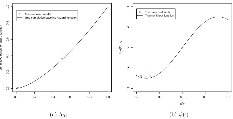
interest, such as the linear covariate parameter β, the nonlinear covariate parameter α and the association parameter φ. The estimate of the cumulative baseline hazard function Λ0(∙) and the nonlinear function ψ(∙) are also given. The second simulation

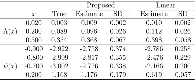
study compares the proposed model with what is referred to as the PH linear model here. The PH linear model is the one that has the same structure as the proposed

model except that the covariates are all assumed to have linear effects on the log

Flexible Partially Linear Single Index Regression Models for Multivariate Survival Data

Flexible Partially Linear Single Index Regression Models for

Flexible Partially Linear Single Index Regression Models for

Multivariate Survival Data

Multivariate Survival Data

FLEXIBLE PARTIALLY LINEAR SINGLE INDEX REGRESSION

MODELS FOR MULTIVARIATE SURVIVAL DATA

(Thesis format: Monograph)

by

Na Lei

Graduate Program in Statistical and Actuarial Sciences

A thesis submitted in partial fulfillment

of the requirements for the degree of

Doctor of Philosophy

The School of Graduate and Postdoctoral Studies

The University of Western Ontario

London, Ontario, Canada

c

Contents

List of Figures

Introduction

1.1

Motivation and Problem Description

1.1.1

Colon Cancer Data

1.1.2

Busselton Health Study Data

1.1.3

Problem Description

1.2

Literature Review

1.2.1

Modeling Association in Multivariate Survival Data

1.2.2

Univariate Regression Models for Survival Data

1.2.3

Extensions on Regression Models

1.3

Overview of the Thesis

Chapter 2

Flexible Partially Linear Single

Index Proportional Hazard

Regression Model for Multivariate

Survival Data

2.1

Introduction

2.2

The Proposed Model

2.2.1

Piecewise Constant Approach for Baseline Function

2.2.2

Spline Function Approximation

2.2.3

The Likelihood

2.2.4

Parameter Estimates

2.3

Simulation Studies