On the Complexity of Certain Algebraic and Number Theoretic Problems

(1)

On the Complexity of Certain

Algebraic and Number Theoretic

Problems

A Thesis Submitted

in Partial Fulfillment of the Requirements for the Degree of

Doctor of Philosophy

by

Chandan Saha

to the

DEPARTMENT OF COMPUTER SCIENCE AND ENGINEERING

INDIAN INSTITUTE OF TECHNOLOGY KANPUR

(2)

It is certified that the work contained in the thesis entitled “On the Complexity of Certain Algebraic and Number Theoretic Problems”, by “Chandan Saha”, has been carried out under my supervision and that this work has not been submitted elsewhere for a degree.

(Dr. Manindra Agrawal) Professor,

Department of Computer Science and Engineering Indian Institute of Technology Kanpur

(3)

Synopsis

In this thesis we study the deterministic complexity of three problems belonging to the subject of computational algebra and number theory. These problems are - univariate polynomial factoring over finite fields, large integer multiplication and polynomial identity testing. The choice of these problems is primarily motivated by their fundamental nature as mathematical problems and by their important appli-cations in areas like coding theory, cryptography and complexity theory.

Finding an efficient deterministic algorithm to factor univariate polynomials over finite fields is a long standing open problem. Building on earlier work by Evdoki-mov and Gao, we show that a given polynomial can be factored in deterministic polynomial time, under the assumption of the Extended Riemann Hypothesis, un-less the roots of the polynomial satisfy a strong symmetry property. Our symmetry property strengthens the symmetry property (square balance) defined by Gao. We also give a tight estimate of the fraction of square balanced polynomials (over fields of characteristic p = 3 mod 4), showing it to be exponentially small. Our main motivation behind this approach to factoring is that checking for inherent asym-metries among the roots can be used to improve the time complexity of the best deterministic algorithms on most input polynomials.

Integer multiplication is ubiquitous in computational number theory. We give an n·logn·2O(log∗n) _{time algorithm to multiply two} _n _{bit integers that uses} mod-ular arithmetic for intermediate computations instead of arithmetic over complex numbers as in F¨urer’s algorithm, which also has the same and so far the best known complexity. The previous best algorithm using modular arithmetic (by Sch¨onhage and Strassen) has complexity O(n·logn·log logn). The advantage of using mod-ular arithmetic as opposed to complex arithmetic is that we can completely evade

(4)

Polynomial Identity Testing (PIT) is a fundamental problem lying at the in-terface of complexity theory and computational algebra. We study the problem of identity testing for depth-2 arithmetic circuits over matrix algebra. We show that identity testing of depth-3 (ΣΠΣ) arithmetic circuits over a field _F is polynomial time equivalent to identity testing of depth-2 (ΠΣ) arithmetic circuits over U2(F), the algebra of upper-triangular 2×2 matrices with entries from _F. Such a con-nection is a bit surprising since we also show that, as computational models, ΠΣ circuits over U2(F) are strictly ‘weaker’ than ΣΠΣ circuits over F. The equivalence further implies that PIT of ΣΠΣ circuits reduces to PIT of width-2 commutative Algebraic Branching Programs(ABP). Further, we give a deterministic polynomial time identity testing algorithm for ΠΣ circuits of size s over commutative algebras of dimension O(logs/log logs) over _F. Over commutative algebras of dimension O(s), we show that identity testing of ΠΣ circuits is at least as hard as that of ΣΠΣ circuits over _F.

Finally, we study the complexity of two particular problems on identity testing. One is a generalization of a problem considered by Kayal and Saxena. Here, we are required to test if the output of a given depth-3 circuit with bounded top fanin equals a given sparse polynomial. The second problem is on checking if a given sparse polynomial equals the product of a given set of other sparse polynomials, a problem that is noted as an open question by von zur Gathen. Using a technique called dual representation of polynomials, we give deterministic polynomial time solutions for the first problem and a special case of the second problem where every polynomial in the input set of alleged factors is a sum of univariate polynomials.

(5)

Acknowledgements

I am deeply thankful to my advisor Manindra Agrawal for his invaluable guidance and his persistent encouragement throughout the course of this work. His interest in solving fundamental problems, his perseverance in the face of failures, and his pursuit for clarity have always inspired me. Much of the work done in this thesis is greatly influenced by his own views, thoughts and ideas. Thank you Manindra, for all your support. I owe a lot to you, not only for your scientific advice but also for all the generous helps that I have received from you throughout these years.

Studying at IIT Kanpur has been an enjoyable experience for me. I am indebted to the faculties of the Department of Computer Science and Engineering, specially Somenath Biswas, Sumit Ganguly, Piyush Kurur and Surender Baswana for their teaching and their many motivational advice that helped me focus on my work. Piyush has also co-authored the work presented in Chapter 4 and I have enjoyed countless hours of stimulating discussions with him which sometimes went into the realm of philosophy :).

I am grateful to Nitin Saxena for the opportunity to visit Hausdorff Center for Mathematics which started the collaborative work described in Chapter 5. The work presented in Chapter 6 is also done in collaboration with Nitin. I must admit, I have learnt quite a bit of algebra from many hours of illuminating discussions with him. His enthusiasm for algebraic methods is inspiring. I also thank him for his hospitality during my stay in Bonn.

Thanks to my colleagues and friends Anindya De and Ramprasad Saptharishi with whom I have collaborated with for the work in Chapter 4. A special thanks to Ramprasad with whom I have had many hours of insightful conversations. I do appreciate his clear thinking and simple ways of expressing non-trivial ideas.

(6)

during my stay in Bonn. I am also very much thankful to Joachim von zur Gathen for kindly inviting me to give a talk at b-it, where I also enjoyed a brief but elucidating conversation with Joachim and Dima Grigoriev on the work in Chapter 4. Thanks to Martin F¨urer for generously sharing his views on his integer multiplication algorithm and also for pointing out a mistake in referring a paper in our work.

I would also like to thank Comandur Seshadhri for explaining to me his work on identity testing with Nitin Saxena, to Srikanth Srinivasan for stimulating conver-sations on complexity theory, to Hendrik W. Lenstra for an e-mail communication (with Manindra) clarifying our doubt regarding existence of a certain result in the literature, and to Andrew Yao and Jayalal Sarma for kindly inviting me to a work-shop at Tsinghua University. A special thanks to Neeraj Kayal for sharing with me his insights on several interesting problems, and for kindly inviting me to visit Microsoft Research India. Thanks to Samiran Chattopadhyay from Jadavpur Uni-versity, the institute of my undergraduate study, for inspiring us to work sincerely.

Many thanks to the anonymous referees who have kindly taken some time out to review this work - their suggestions have improved the presentation of this thesis.

Life at IIT would not have been the same without my friends around me and I feel fortunate to have a good many of them. Without naming them individually, I express my deepest gratitude to all of them for making my stay in IIT a memorable one. Still I feel compelled to especially thank Deepanjan Kesh and Ramprasad Saptharishi for being always there to cheer me up. And thanks also to my office-mate Purushottam Kar - his sincerity is contagious.

Finally, it was all made possible for me by my family’s continual and uncon-ditional love and support. I thank my sister for her love and care, and also for originally instilling in me an interest for research. Thanks to my brother (in-law) for being a wonderful person whom I have always found refreshing to talk to. I am deeply indebted to my parents for being what they are, for loving me, caring for me and encouraging me to pursue whatever I am interested in. I do not know whether it is possible for me to return an iota of what I have received from them - perhaps it is not. Still, I will feel content to dedicate this little piece of work to them, and I do so with humility.

(7)

(8)

(9)

Chapter 1

Introduction

Much of our endeavor in the theoretical study of computation is aimed towards either finding an efficient algorithm for a problem or gauging the hardness of a problem. And in meeting both these goals mathematical insights and ingenuities are constant companions. In particular, two branches of mathematics - combinatorics, and algebra and number theory, have found extensive applications in theoretical computer science. In this thesis, our focus is on problems belonging to the latter branch.

For the past few decades there has been a growing interest among computer scientists and mathematicians, in the field of computational number theory and algebra. Computational number theory is the branch of computer science that involves finding efficient algorithms for algebraic and number theoretic problems. Since its inception in the early 1960s, this field has continued to grow with ever-rising interest among researchers from diverse disciplines that resulted in a fruitful union of different areas in mathematics and computer science, especially algebra, number theory and computational complexity theory.

Factoring large integers, checking if an integer is prime, factoring polynomials, multiplying large integers and matrices, and solving polynomial equations are a few among a plethora of problems that have made this area so rich and fascinating. Unlike numerical analysis, here we are interested in exact solutions to problems instead of approximate solutions. Owing to the fundamental nature of the problems involved, this is a subject of intense theoretical pursuit. And the tools and techniques developed to solve these problems have provided researchers with deep mathematical

(14)

insights. But interest in them has escalated in recent time because of their important applications in key areas like cryptography, coding theory and complexity theory.

To cite a few examples, the security and efficiency of cryptographic protocols such as the RSA cryptosystem and the Diffie-Hellman key exchange protocol, rely on the hardness of problems like integer factoring and discrete logarithm and on the efficiency of prime number generation and large integer multiplication. Further, the efficiency of some of the decoding algorithms for error correcting codes like Reed-Solomon and BCH codes, hinge on fast algorithms for solving a system of linear equations and factoring polynomials over finite fields. Another important application of algorithmic algebra is the development of computer algebra systems. These systems are indispensable tools for research in many computation intensive fields of physics, chemistry, biology, mathematics, geology and meteorology.

The basic computer algebra operations can be broadly classified as

-• Polynomial operations: Polynomial addition, multiplication, gcd computa-tion, factoring, interpolacomputa-tion, multipoint evaluacomputa-tion, identity testing.

• Integer operations: Addition, multiplication, gcd computation, square root finding, primality testing, integer factoring, etc.

• Linear algebra operations: Matrix addition, multiplication, inverse and determinant computation, solving a system of linear equations, etc.

• Abstract algebra operations: Finding the order of a group element, com-puting discrete logarithm, etc.

In this thesis, we study three such operations namely, univariate polynomial fac-toring over finite fields, large integer multiplication and polynomial identity testing. Our attempt in understanding the computational complexity of these problems is driven both by the fundamental nature of these problems as well as by their strik-ing applications in other areas. In this chapter we formally define these problems, noting alongside a few motivating applications. We then give an overview of our results with the intent of placing them in the context of earlier work.

(15)

1.1 The Problems 3

1.1

The Problems

We now state the problems that we work with in this thesis. Definition of a finite field can be looked up from Section 2.1.1in Chapter 2.

Problem 1.1.1. (Polynomial factoring) Given a univariate polynomial f of degree n with coefficients taken from a finite field _Fq, the field with q elements, find all the irreducible factors of f.

Polynomial factoring is a fundamental problem that has been studied by the research community for over four decades. So far there is no known deterministic polynomial time solution. Polynomial f is given as an input in terms of all its n coefficients. Since _Fq has q elements, each coefficient can be represented by about dlogqebits. So a polynomial time algorithm must run in time (nlogq)c_{, where}_c_{is an} absolute constant independent ofn and logq. Problem1.1.1 is known to admit effi-cient randomized polynomial time algorithms (Ber67;Ber70;vzGS92;KS98;KU08). However, the popular belief is that ‘a problem with a randomized polynomial time solution can also be solved in deterministic polynomial time’ and hence our focus is on deterministic solutions to Problem 1.1.1.

Polynomial factoring finds important applications in coding theory, as in the list decoding algorithms of Reed-Solomon codes (Sud97; GS99), and also in designing efficient algorithms for other algebraic problems like polynomial solvability (Kay05;

KY08).

Our second problem is integer multiplication.

Problem 1.1.2. (Integer multiplication) Find an efficient algorithm to multiply two n-bit integers.

The high school algorithm to multiply two integers is efficient when the integers involved are small, but it quickly becomes inapplicable for larger integers. Multi-plication of large integers do arise in practice. For example, the RSA encryption process starts by multiplying two large primes. Many other cryptosystems also require to generate large primes, and choosing primes is usually accompanied by primality testing. The only known deterministic polynomial time primality test is the AKS family (AKS04) of tests. Crandall and Papadopoulos (CP03) remarked on

(16)

their AKS implementation, “...in our implementation almost all of the time is spent multiplying (and squaring) large integers.”

Our third problem is polynomial identity testing. Arithmetic circuits are defined in Section 2.1.2 of Chapter 2.

Problem 1.1.3. (Polynomial Identity Testing) Given an arithmetic circuit C with input variables x1, . . . , xn and constants taken from a fieldF, check if the polynomial

f(x1, . . . , xn) computed by C is identically zero.

Beside being a natural problem in algebraic computation, identity testing ap-pears in important complexity theory results such as, IP = PSPACE (LFKN90;

Sha90) and the PCP theorem (ALM+98). It also plays a promising role in proving super-polynomial circuit lower bound for the permanent polynomial (KI03; Agr05). Moreover, algorithms for problems like primality testing (AKS04), graph matching (Lov79) and multivariate polynomial interpolation (CDGK91) also involve identity testing. Several efficient randomized algorithms (Sch80; Zip79;CK97; LV98; AB99;

KS01) are already known for identity testing. However, a deterministic polynomial time algorithm has remained elusive. In this thesis, we are particularly interested in a special case of identity testing that has received a lot of attention in recent times. This is the problem of identity testing for circuits of depth 3.

We now move on to give a summary of our contributions to the above mentioned problems.

1.2

Our Contributions

The purpose of this section is to present a brief overview of our results, all of which are directed towards finding efficient deterministic algorithms for the problems stated in the previous section. The definitions of the basic terminologies, like algebra, endomorphism, zero-divisor, Fourier transform, circuits, etc., can be looked up from Sections2.1 and 2.3 in Chapter 2.

(17)

1.2 Our Contributions 5

1.2.1

Factoring Polynomials using Balance Test

As stated before, univariate polynomial factoring over finite fields is yet to be solved in deterministic polynomial time, even under the powerful assumption of the Ex-tended Riemann Hypothesis (ERH). Without the assumption of the ERH, it is not even known how to efficiently find square root of an element a∈ _Fp, which can be equivalently thought of as factoring polynomial x2₋_{a. The results in this section} assume the validity of the ERH.

The best deterministic factoring algorithm, due to Evdokimov (Evd94), runs in time polynomial in nlogn _{and log}_{p, where} _n _{is the degree of the input polynomial} f(x) andpis the characteristic of the finite field_Fp. Evdokimov’s algorithm involves finding factors of polynomials of ‘smaller’ degree but with coefficients coming from algebras of dimension O(nlogn) over _Fp. Using these factors eventually a nontrivial endomorphism of the ringR= Fp[x]

(f) is found, or in the process a zero-divisor of Ris encountered. Evdokimov showed that both these cases are sufficient to factor f.

An alternative approach, due to Gao (Gao01), is to exploit an inherent asym-metry among the n roots of f to find a zero-divisor in R. This approach has its merit as it avoids computation in algebras of superpolynomial dimension over _Fp. However, Gao’s algorithm fails to factorf if its roots satisfy a symmetry condition, known as square balance. Square balanced polynomials do exist, although we show in our work that the fraction of such polynomials is exponentially small in n over fields of characteristic p= 3 mod 4.

In our work (Sah08), we propose an extension of Gao’s algorithm in a way that attempts to bring together the merits of both Evdokimov’s and Gao’s approaches. Our primary motivation in unifying the two approaches lies in the following informal observation. If the number of roots, i.e. n is ‘large’ then they are ‘unlikely’ to sat-isfy a sufficiently strong symmetry condition. Else, if n is small then Evdokimov’s algorithm is efficient by itself. We briefly sketch how this observation is put to work.

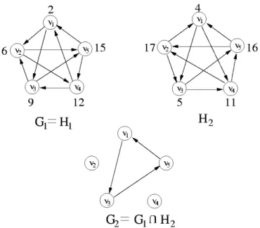
Our algorithm (implicitly) constructsk simple digraphsG1, . . . , Gk onnvertices (labelled 1, . . . , n) such thatG` is a subgraph (not necessarily a proper subgraph) of G`−1. There is an edge (i, j) in G` if the difference of theith and the jth roots of f satisfy a ‘certain’ condition. We show that if any of the k graphs is not regular (i.e.

(18)

indegree and outdegree not same for all vertices) then a zero-divisor of R is found. Otherwise, if all the graphsG1, . . . , Gk are regular then we require at most log₂n of the graphsG` to be such thatG` 6=G`−1, so that a nontrivial endomorphism ofRis obtained. As mentioned earlier, by the work of Evdokimov (Evd94), a zero-divisor or an endomorphism in turn produces a factor of f. The time complexity of our algorithm isk·(nlogp)O(1)_{. The graph} _G

1 is regular exactly for the class of square balanced polynomials, which makes the test that G1, . . . , Gk are regular (we call, balance test) stronger than Gao’s test.

The construction of the graphs is flexible in the sense that any arbitrary but deterministically chosen auxiliary polynomialsq1(y), . . . , qk(y) of degree (nlogp)O(1) can be used to form the graphs. For instance, by choosing q`(y) = (y+ 2−1`)2 a bound of k ≤ √plogp can be shown for p = 3 mod 4, so that our algorithm always succeeds in factoring f for this value of k. However, the task is to show better bounds on k and we leave this question open, noting that for a random choice of q`(y), G` 6= G`−1 with high probability. The ideal goal is to show that k = (nlogp)O(1) by appropriately fixing the auxiliary polynomials, in which case factoring polynomials under ERH can be solved in deterministic polynomial time.

Theorem 1.2.1. Univariate polynomials over finite fields can be factored in deter-ministic polynomial time, under the assumption of the ERH, unless the roots of the polynomial satisfy a strong symmetry condition.

1.2.2

Integer Multiplication using Modular Arithmetic

How fast can we multiply twon-bit integers? In a seminal paper (SS71), Sch¨onhage and Strassen gave two algorithms to multiply integers - one having a time com-plexity of O(n ·logn· log logn . . .2O(log∗n)_{) bit operations, and another having a} complexity of O(n ·logn ·log logn) bit operations. The first algorithm involves arithmetic over complex numbers while the second one uses modular arithmetic. However, both these algorithms are based on one central theme - reduce integer multiplication to polynomial multiplication and then multiply the polynomials us-ing Fast Fourier Transform. The main technical step here is to suitably encode the integers as polynomials over a ring that has a ‘good’ principal root of unity which is crucial in making Discrete Fourier Transform (DFT) efficient.

(19)

After a period of dormancy in progress, Fürer came up with a breakthrough re-sult (Für07) that multiplies twon-bit integers usingn·logn·2O(log∗n)_{bit operations.} While Fürer’s overall approach remains the same as in (SS71), he quite importantly introduced the notion of inner and outer DFT and showed how repeated compu-tation of inner DFTs, efficiently, leads to an overall saving in time. For the inner DFT idea to work, an appropriate root of unity is required which is less of an issue here as the underlying field of complex numbers is algebraically closed. However, all intermediate complex numbers need to be approximated suitably during compu-tation and this introduces the added task of bounding the total truncation error in the analysis of the algorithm. The question that motivated us is - Can we dispense with the elaborate error analysis by giving a ‘discrete’ adaption of Fürer’s algorithm?

In our work (DKSS08), we show that two n-bit integers can be multiplied in n ·logn ·2O(log∗n) _{time using modular arithmetic. Our algorithm closely follows} Fürer’s algorithm, but departs from it by using modular arithmetic for intermedi-ate computations instead of complex arithmetic. The primary technical hurdle here is to make the inner DFTs efficient while working over a discrete ring. This we overcome by invoking a deep result in analytic number theory on the least prime in an arithmetic progression (Linnik’s theorem), and by using FFT over multivariate polynomials as opposed to univariate-FFT, which is the case in both Fürer’s and Schönhage-Strassen’s algorithms. This also means that the notion of inner and outer DFT has to be translated properly to make it work in the multivariate world. Over-all, the algorithm becomes more transparent and simple (without any truncation error analysis), making it plausible that a suitable variant of it might lead to an O(nlogn) algorithm, thereby matching the popular belief on integer multiplication complexity.

Theorem 1.2.2. There is ann·logn·2O(log∗n)_{time algorithm to compute the product} of two n bit integers using only modular arithmetic for intermediate computations.

1.2.3

Identity Testing via Depth

2

Circuits over Algebras

Recall that, Polynomial Identity Testing (PIT) is the problem of efficiently decid-ing if a multivariate polynomial given as an arithmetic circuit is identically zero.

(20)

The goal is to find a deterministic polynomial time algorithm. One specific case of PIT is identity testing for depth-3 (ΣΠΣ) arithmetic circuits. In the last few years depth-3 PIT has been intensely studied (DS05; KS07; SS09; KS09; SS10b; SS10a) by the research community. The best result known along this line of research is a deterministic polynomial time ‘blackbox’ algorithm for PIT of ΣΠΣ circuits with bounded top fan-in. However, PIT of general ΣΠΣ circuits remains a long standing open problem.

In our work (SSS09), we take a different approach to depth-3 identity testing by reducing the depth of the circuit to 2 while increasing the dimension of the underlying algebra. We show that identity testing of depth 3 (ΣΠΣ) arithmetic circuits over a field _F is polynomial time equivalent to identity testing of depth 2 (ΠΣ) arithmetic circuits overU2(F), the algebra of upper-triangular 2×2 matrices with entries from _F. Such a connection is a bit surprising since we also show that, as computational models, ΠΣ circuits over U2(F) are strictly ‘weaker’ than ΣΠΣ circuits over _F. The equivalence further implies that PIT of ΣΠΣ circuits reduces to PIT of width-2 commutative Algebraic Branching Programs(ABP). This is in contrast to the fact that identity testing of any ‘non-commutative’ ABP can be done in deterministic polynomial time (RS04) and the reduction justifies to some extent the lack of progress for commutative ABPs.

We also show that PIT of a depth-3 circuit of sizesreduces in polynomial time to PIT of a depth-2 circuit of sizeO(s) over a commutative algebra of dimensionO(s). We make some progress along this line by giving a deterministic polynomial time identity testing algorithm for depth-2 circuits of size s over commutative algebras of dimension O(logs/log logs). The main technical ingredient of our algorithm is an effective version of a structure theorem that states that a finite dimensional commutative algebra splits into local rings.

Thus, if we can extend the above result toO(s) dimension or use deeper algebraic insight into the ring of 2×2 matrices to solve PIT of ΠΣ circuits over U2(F), then

depth-3 PIT can be solved in polynomial time.

Theorem 1.2.3. (a) Identity testing of depth-3 circuits is polynomial time equiv-alent to identity testing of depth-2 circuits over 2× 2 upper-triangular matrices,

(21)

although the latter model is ‘computationally weaker’ than the former.

(b) Also, PIT of depth-3 circuits of size s reduces to PIT of depth-2 circuits of size O(s)over commutative algebras of dimensionO(s). There is a deterministic polyno-mial time identity testing algorithm for depth-2 circuits of size s over commutative algebras of dimension O(_{log log}logs_s).

1.2.4

Applying Duality to Two Identity Testing Problems

Finally, we study the complexity of two particular problems on identity testing. The first problem is a natural generalization of a problem on depth-3 identity testing studied before by Kayal and Saxena (KS07).

Problem 1.2.4. Given a depth-3 circuit C with bounded top fanin and given a sparse polynomial f explicitly, check if p(C) = f, where p(C) is the polynomial computed by C.

Kayal and Saxena (KS07) showed that identity testing of a depth-3 circuit with bounded top fanin can be solved in deterministic polynomial time, which thereby solves the case when f = 0 in Problem 1.2.4 (Recently, Saxena and Seshadhri (SS10a) gave a blackbox polynomial time algorithm to check ifp(C) = 0). We gen-eralize their result using a technique known as dual representation of polynomials (introduced in (Sax08)), to show that Problem1.2.4 can be solved in deterministic polynomial time for any given sparse polynomial f.

The second problem we study is also a very natural case of identity testing.

Problem 1.2.5. Given a polynomialf explicitly, and also givent other polynomials g1, . . . , gt explicitly (gi’s need not be distinct), check if f =g1. . . gt.

This problem has been mentioned in a work by von zur Gathen (vzG83) as a problem with no known efficient deterministic solution. Using the same tool of ‘duality’, we give a deterministic polynomial time algorithm to solve Problem 1.2.5 for the case when the input factors g1, . . . , gt are of the form of sum of univariates.

Roughly speaking, duality is an efficient technique to express a polynomial of a special kind, we call a semidiagonal polynomial, as a ‘small’ sum of product of univariates. This particular representation of semidiagonal polynomials turns out to be quite useful in solving both the above problems.

(22)

1.3

Organization

The rest of the thesis is organized as follows. In Chapter 2we give a brief overview of the basic algebraic concepts and tools used in our work. Chapter 3and Chapter 4 are devoted to our results on polynomial factoring and integer multiplication, respectively. The results on identity testing are covered in Chapter 5 and Chapter 6.

(23)

Chapter 2

Preliminaries

In this chapter we give a concise introduction to the basic mathematical constructs and tools that we allude to throughout the rest of this thesis. In the first section, we define the algebraic and the computational structures and note some of their relevant properties. While in the second section, we provide a more or less self contained exposition to some of the standard mathematical tools that play an important role in our results. The details provided in this section are primarily for completeness and the reader’s convenience.

2.1

Basic Structures

2.1.1

Rings and Fields

In this section, we collect the definitions of some of the basic algebraic structures, often accompanying them with simple representative examples. Extensive treatment of these concepts can be found in any standard textbook (Lan02; DF99; Her75;

Art91) on abstract algebra.

Definition 2.1.1. (Group) A group G is a set of elements along with a binary op-erator

.

that satisfies the following properties

-1. (Closure) For every two elements a, b∈G, a

.

b also belongs to G. 2. (Associativity) For every three elements a, b, c∈G, (a

.

b)

.

c=a

.

(b

.

c).

(24)

3. (Identity) There is an element e∈G such that for all a, a

.

e=e

.

a=a. 4. (Inverse) Every element a has an inverse b ∈G satisfying a

.

b=b

.

a=e.

Example - (Symmetric groups) The set of all bijections from a set onto itself is a group, where the binary operator

.

is composition of mappings.

A group, often written as a tuple (G,

.

), is commutative or abelian if for every a, b ∈ G, a

.

b = b

.

a. If G satisfies only the closure and the associativity properties under

.

, then (G,

.

) is called asemigroup.

Definition 2.1.2. (Ring) A ring R is a set of elements along with two binary oper-ators + and

.

such that

-1. (R,+) is an abelian group.

2. (R− {0},

.

) is a semigroup, where 0 is the identity of (R,+).

3. For every a, b and c∈R, (a+b)

.

c=a

.

c+b

.

cand a

.

(b+c) = a

.

b+a

.

c.

Example- (Integer and polynomial ring) The set of integers _Zand the set of poly-nomials with integer coefficients_Z[x] are rings under normal integer and polynomial addition and multiplication, respectively.

Some ring-theoretic concepts - A ring R is commutative if for all a, b ∈ R, a

.

b = b

.

a. Ring R is said to have a unity, if there is an element e ∈ R for which a

.

e = e

.

a = a, for all a ∈ R. By convention, the unity in R is denoted by 1 and the identity element of (R,+) is denoted by 0. An element a 6= 0 is a zero divisor if there exist a b 6= 0 such that a

.

b = 0; and a is nilpotent if an = 0 for a positive integer n. A commutative ring with no zero divisor is called an integral domain. Elements, in a ring R with unity, which are invertible in (R− {0},

.

) are called units. For two different rings (R1,+,

.

) and (R2,+,

.

), although we use the same notation to denote the different rings operations + and

.

, they should be interpreted appropriately from the context of their usage. The direct sum of two rings R1 and

R2, denoted as R1 ⊕R2, is a ring R with elements of the form r = (r1, r2) for all r1 ∈R1 and r2 ∈R2. Addition and multiplication in R is defined as componentwise addition and multiplication over R1 and R2 i.e. ifr = (r1, r2) and r0 = (r01, r02) then

(25)

2.1 Basic Structures 13

r+r0 = (r1 +r₁0, r2 +r0₂) and r

.

r0 = (r1

.

r₁0, r2

.

r₂0). Surely, this definition extends to direct sum of multiple rings.

Definition 2.1.3. (Ring homomorphism) A mapping φ from a ring (R1,+,

.

) to a ring (R2,+,

.

) is a ring homomorphism if for every a and b in R1,

1. φ(a+b) = φ(a) +φ(b). 2. φ(a

.

b) =φ(a)

.

φ(b). 3. φ(1) = 1.

The set of elements of R1 which map to the element 0 in R2, under the action of a ring homomorphism φ, is called the kernel of φ denoted by ker(φ). When a ring homomorphismφ is one-one and onto, it is called an isomorphism and the rings are then said to beisomorphic. A homomorphism fromRto itself is called an endomor-phism, and an endomorphism that is also an isomorphism is called anautomorphism.

Example- (Residues modulon) Given a positive integern, let_Z/n_Z={0, . . . , n−1} be the ring of residues under addition and multiplication modulo n. Then the map which takes a∈ _Z toa (mod n) i.e. the (positive) remainder when a is divided by n, is a ring homomorphism from _Z to_Z/n_Z.

Definition 2.1.4. (Ideal) A subset I of a ring (R,+,

.

) is an ideal of R if (I,+) is a subgroup of (R,+) and for every a∈I and b∈R, b

.

a and a

.

b belong to I. An ideal of R which is not properly contained in any ideal other than R itself, is called a maximal ideal. We say that an ideal I is generated by the elements a1, . . . , ak ∈I, denoted asI= (a1, . . . , ak), if and only if everyb∈Ican be expressed as b=b1

.

a1+. . .+bk

.

ak where bi’s belong to R.

Definition 2.1.5. (Quotient ring) Given an ideal I of a ring R, the quotient ring

R/Iis defined on the set of elements{a+I|a ∈R} satisfying the following relations for all a, b∈R :

1. a+I=b+I if and only if a−b∈I. 2. (a+I) + (b+I) = (a+b) +I.

(26)

3. (a+I)

.

(b+I) = (a

.

b) +I.

Example - The set of integer multiples of a number n ∈ _Z, denoted as n_Z, is an ideal of _Z. If n is a prime then n_Z is a maximal ideal. The ring _Z/n_Z of residues modulo n is a quotient ring with respect to the ideal n_Z.

Definition 2.1.6. (Primitive root of unity) Let R be a commutative ring with unity 1. An element ω ∈ R is called a primitive nth _{root of unity if} _ωn _{= 1, the element} n= 1 + 1 +. . . n times is a unit in R, and for every 1≤m < n, ωm₋₁ _{is nonzero} and not a zero divisor.

Observation 2.1.7. If ω is a primitive nth _{root of unity in} R _{then for every} ₁ _≤ m < n, Pn−1

j=0 ωmj = 0.

Proof. Notice that, (ωm −1)·Pn−1

j=0 ω

mj ₌ _ωmn ₋_{1 = 0 and} _ωm₋₁ _{6= 0 is not a} zero divisor, implying that Pn−1

j=0ω

mj _{= 0.}

Example- In the ring _Z/5_Z, the element 2 is a primitive 4th _{root of unity.}

Definition 2.1.8. (Local ring) A commutative ring R is local if it has a unique maximal ideal.

Example - Let R = _Q[x] be the ring of univariate polynomials in x with rational coefficients, and xnR be the ideal of all polynomials that are divisible by xn, where n is a positive integer. Then the quotient ring R/xnR _{is a local ring with exactly} one maximal ideal consisting of all polynomials that are divisible by x.

Definition 2.1.9. (Field) A ring (R,+,

.

) is a field if (R− {0},

.

) is an abelian group. In other words, a commutative ring R with unity is a field if every nonzero element in R is invertible.

Example- (Polynomial ring and rational functions) The sets of rationals, reals and complex numbers are fields. The set of polynomials in the indeterminatesx1, . . . , xn with coefficients taken from a field _F, denoted as _F[x1, . . . , xn], is a ring under ‘natural’ polynomial addition and multiplication. This is called thepolynomial ring. Then the set _F(x1, . . . , xn) = {f /g : f, g ∈ _F[x1, . . . , xn] and g 6= 0} is a field also known as the field of rational functions or the quotient field of the polynomial ring.

(27)

Definition 2.1.10. (Finite field) A field with finite number of elements is called a finite field.

Example - For every prime p, the quotient ring _Z/p_Z is a field consisting of p elements. Let _F be a finite field with q elements and f(x) ∈ _F[x] be an irreducible polynomial (see the definition below) of degree n. Then _F[x]/(f) is a field with qn elements, where (f) is the ideal of_F[x] consisting of all multiples of f.

Ifpis the prime for which 1+1+. . . p times = 0 in_Fthenpis called thecharacteristic of _F. If no such prime exists then field_F is said to have zero characteristic.

Definition 2.1.11. (Unique factorization domain) Let R be an integral domain with unity. An element p∈ R is irreducible if whenever p=a

.

b with a, b ∈R, either a or b is a unit. Ring R is a unique factorization domain if every nonunit r∈R can be uniquely expressed as a finite product of irreducible elements. The uniqueness of the product is up to multiplication by units.

Example- The polynomial ring_F[x1, . . . , xn] over a fieldFis a unique factorization domain where every polynomial can be factored uniquely into irreducible factors.

Definition 2.1.12. (Vector space) A commutative group (V,+) is a vector space over a field _Fif for every a∈_F andv ∈V there is an element av ∈Vsatisfying the following relations. For all a, b∈_F and v, w∈V,

1. a(v+w) =av+aw. 2. (a+b)v =av+bv. 3. a(bv) = (ab)v. 4. 1v =v.

Example - The polynomial ring _F[x1, . . . , xn] is a vector space over F. The set of n×n matrices with entries from a field _F, denoted as Mn(F), is also a vector space over _F. Also, the set of complex numbers is a vector space over reals.

Vectors v1, . . . , vm ∈ V are said to be linearly independent if any vector of the form a1v1+. . . amvm, with ai’s in F, cannot be 0 unless every ai is zero. Elements

(28)

e1, . . . , en ∈ V are said to form a basis of V if every v ∈ V can be expressed as a1e1 +. . . anen, where ai’s in F are unique depending only on v. In this case, n is called the dimension of the vector space V.

Definition 2.1.13. (Algebra over fields) A ring (A,+,

.

) is called an algebra over a field _F if (A,+) forms a vector space over _F and for every v, w ∈ A and a ∈ _F, a(v

.

w) = (av)

.

w=v

.

(aw).

Example - The quotient ring _F[x]/(f), where f is a polynomial of degree n is an algebra over _F of dimension n. The set ofn×n matrices, Mn(F), forms an algebra over _Fof dimension n2_.

We say that an_F-basis of an algebra isexplicitly given if we know the basis elements (say) {e1, . . . , en} and we also know how ei

.

ej expands as an F-linear combination of {e1, . . . , en}, for every i and j. The direct sum of two algebras A1 and A2 is an algebraA=A1⊕A2, which is the same as the direct sum of rings A1 and A2 with the added property that if v = (v1, v2), where v1 ∈ A1, v2 ∈ A2 and v ∈ A, then av= (av1, av2) for every a∈F.

2.1.2

Arithmetic Circuits

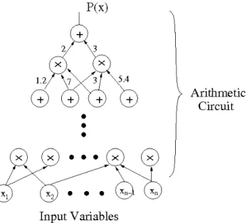
Arithmetic circuits form a natural model for computing multivariate polynomials. It is the arithmetic analogue of boolean circuits, the nonuniform version of Turing machines. Problems involving arithmetic circuits, in particular proving explicit cir-cuit lower bounds, have been studied since the early 70s. Formally, an arithmetic circuit is defined as follows.

Definition 2.1.14. (Arithmetic circuit) An arithmetic circuit over a field _F is a directed acyclic graph with nodes labelled by the two operations + and ×, while nodes with indegree zero are labelled by the input variables x1, . . . , xn and by field elements. The edges are labelled only by field elements (no label indicates a label by 1). Circuit C computes polynomials in _F[x1, . . . , xn] in a natural way. The output of nodes labelled by xi (or, a constant) are xi (or, the constant). An edge (v, w) which is labelled by α ∈ _F multiplies the output of v with α and feeds in to the input of w. Nodes labelled by + and × output the sum and the product of the

(29)

corresponding input polynomials, respectively. Nodes with outdegree zero output the final polynomials computed by the circuit.

The following figure shows an example of a circuit. The size of a circuit is the total number of nodes and edges in the underlying directed graph. The depth of a circuit is the length of the longest path from an input to an output node. A circuit is called a formula if every node has outdegree at most one.

Figure 2.1: An arithmetic circuit.

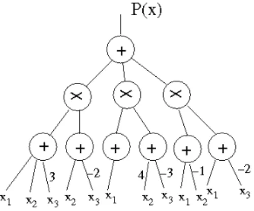
Bounded depth circuits- An infinite family of circuits whose depths are bounded by a constant is called a family of bounded depth circuits. Interestingly enough, bounded depth circuits capture a great deal about circuits in general. This point will be explained in Chapter 5. The following is an example of a depth-3 circuit computing the polynomial (x1+x2+3x3)(x2−2x3)+x1(4x2−3x3)+(x1−x2)(x1−2x3). The fanin of the topmost ‘+’ gate is called the top fanin of the depth-3 circuit. In this case, the top fanin is 3. In Chapter 5 we will be interested in identity testing of depth-3 circuits.

(30)

Figure 2.2: A depth-3 circuit.

2.2

Notations and Conventions

Useful sets

The sets of integers, rationals, reals and complex numbers are denoted by _Z,_Q,_R and _C, respectively. _Z+ _{is the set of positive integers and}

ZN is the ring of integers modulo N ∈_Z+_{. The multiplicative subgroup of}

ZN, consisting of all m∈Z+ with

gcd(m, N) = 1, is denoted by _Z×_N. _F represents any arbitrary field, and _Fq is the finite field with q elements. _F×_q =_Fq\{0}is the multiplicative subgroup of Fq.

The Order notation

Given two functions t1(n) and t2(n) from Z+ → Z+, we write t1(n) = O(t2(n)) if there exist positive constants c and n0 such that t1(n)≤c·t2(n) for every n ≥n0. We write t1(n) = o(t2(n)) if for every constant c, there is an n0 > 0 such that t1(n)< c·t2(n) for all n ≥n0. We use the notation poly(n1, . . . , nk) to mean some arbitrary but fixed polynomial in the parametersn1, . . . , nk. Throughout this thesis, log refers to logarithm base 2 and ln is the natural logarithm. Sometimes, for the sake of brevity we use the notation ˜O(t(n)) to mean O(t(n)·poly(logt(n))).

Other conventions

In this thesis, a ring R always means a commutative ring with unity 1. We write

(31)

2.3 Basic Tools 19

a field _F is denoted by char(_F). Given two polynomials f, g ∈ _F[x], where _F is any field, gcd(f, g) refers to the unique monic largest common divisor of f and g over _F. For any f ∈ _F[x], f0 denotes the formal derivative of f with respect to x i.e. _dxdf. For a positive real a, bac is the largest integer less than a, and dae is the smallest integer greater thana. The determinant of a square matrixM is denoted by det(M). Given two polynomials f, g ∈R[x], where R is an integral domain, S(f, g) denotes the Sylvester matrix of f and g over R. The resultant off and g overR is Resx(f, g) = det(S(f, g)). Refer to Appendix A.1, for a discussion on resultant.

2.3

Basic Tools

Our results rely heavily on certain fundamental mathematical results ortools, namely - Chinese Remaindering Theorem, Hensel Lifting, Discrete Fourier Transform, and a structure theorem on finite dimensional commutative algebra. This section is devoted to a brief study of these tools. More details on them can be found in the texts (GG03; Sho09; AM69) or in the lecture notes (Sud).

2.3.1

Chinese Remaindering

This is a structural result about rings which is used for speeding up computation over integers and polynomials, and also for arguing over rings as in some of the proofs in Chapter 3. For convenience, we present the theorem in a general form and then apply it to the ring of integers and the ring of polynomials.

Two ideals I and J of a ring R are coprime if there are elements a ∈ I and b ∈ J such that a+b = 1. The product of two ideals I and J, denoted by IJ, is the ideal generated by all elements of the form a·b where a ∈ I and b ∈ J. The theorem states the following.

Theorem 2.3.1. (Chinese Remaindering Theorem)Let I1, . . . ,Ir be pairwise coprime ideals of R and I=I1. . .Ir be their product. Then,

R I ∼= R I1 ⊕. . .⊕ R Ir

(32)

Moreover, this isomorphism map is given by,

a modI−→(a modI1, . . . , amod Ir) for all a∈R.

Proof. The proof uses induction on the number of coprime ideals. Let J=I2. . .Ir. Since I1 is coprime to Ij for every j, 2 ≤ j ≤ r, there are elements yj ∈ Ij and xj ∈I1 such that xj+yj = 1. Therefore, Qr_j=2(xj +yj) =x+y0 = 1 where x∈I1 and y0 ∈J, implying thatI1 and J are coprime.

We claim that I = I1 ∩J. By definition, I = I1J and it is easy to see that

I1J ⊆ I1∩J. If z ∈ I1∩J then, from x+y0 = 1 we have zx+zy0 = z. The left hand side of the last equation is an element ofI1J as both zx, zy0 ∈I1J. Therefore,

I1∩J=I1J=I.

Consider the map φ : R_I → _IR 1 ⊕

R

J defined as φ(a mod I) = (a mod I1, a modJ). It is easy to check that φ is well-defined and is in fact a homomorphism. Let a1 =a mod I1 and a0 =a mod J. We will abuse notation slightly and write φ(a) = (a1, a0).

Ifφ(a) =φ(b) = (a1, a0) thena1 =a modI1 =b modI1, implying thata−b∈I1. Similarly, a−b ∈J. This means a−b ∈I1∩J=I and hence φ is a one-one map. Also, sincex+y0 = 1 forx∈I1 andy0 ∈J, we haveφ(a1y0+a0x) = (a1, a0) implying that φ is onto. Therefore, φ is an isomorphism i.e. R_I ∼= _IR

1 ⊕ R J. Inductively, we can show that R_J ∼= _IR 2 ⊕. . .⊕ R Ir and hence, R I ∼= IR1 ⊕. . .⊕ R Ir.

In _Z(or _F[x]), two elements m1 and m2 are coprime integers (or polynomials) if and only if the ideals (m1) and (m2) are coprime. Applying the above theorem to the ring of integers (or polynomials) we get the following result.

Corollary 2.3.2. Let m ∈ R = _Z (or _F[x]) be such that m = Qr

j=1mj where m1, . . . , mr are pairwise coprime integers (or polynomials). Then _(m)R ∼= _(m1)R ⊕. . .⊕

R

(mr).

Thus every element of the ring _(m)R can be uniquely written as an r-tuple with the ith _{component belonging to the ring} R

(mi). Addition and multiplication in

R

(m) are just component-wise addition and multiplication in the rings _(mR

(33)

2.3 Basic Tools 21

2.3.2

Hensel Lifting

Given a ring R and an element m ∈ R, Hensel (Hen18) designed a method to compute factorization of any element of R modulo m` _{(for an integer} _{` >} _{0), given} its factorization modulo m. This method, known as Hensel lifting, is used in many algorithms including multivariate polynomial factoring and polynomial division. In this thesis, we use this tool in Chapter 4to ‘lift’ a root of unity, as stated in Lemma 2.3.5. Once again, we present the general theorem first and then apply it to prove the case (Lemma 2.3.5) we need.

Lemma 2.3.3. (Hensel lifting)LetIbe an ideal of ringR. Given elementsf, g, h, s, t∈

R with f =gh modI and sg+th = 1 modI there exist g0, h0 ∈R such that, f = g0h0 mod I2

g0 = g modI h0 = h mod I.

Further, any g0 and h0 satisfying the above conditions also satisfy: 1. s0g0 +t0h0 = 1 mod I2 _{for some} _s0 ₌_s _mod _I _and _t0 ₌_t _mod_I_.

2. g0 and h0 are unique in the sense that any other solutions g∗ and h∗ sat-isfying the above conditions also satisfy, g∗ = (1 + u)g0 modI2 and h∗ = (1−u)h0 mod I2, for some u∈I.

Proof. Letf−gh=e mod I2. Verify thatg0 =g+te mod I2 andh0 =h+se mod I2 satisfy the conditions f =g0h0 modI2, g0 =g modI and h0 =h modI. We refer to these three conditions together byC.

For any g0, h0 satisfying C, let d = sg0+th0 −1 mod I2. Verify that s0 = (1− d)s mod I2 and t0 = (1−d)t modI2 satisfy the conditions s0g0 +t0h0 = 1 modI2, s0 =s mod Iand t0 =t modI.

Supposeg∗, h∗ be another solution satisfyingC. Letv =g∗−g0 andw=h∗−h0. The relationg∗h∗ =g0h0 mod I2implies thatg0w+h0v = 0 mod I2, asv, w∈I. Since s0g0+t0h0 = 1 mod I2, multiplying both sides byvwe get (s0v−t0_w)g0 ₌_v _mod_I2_{. By} takingu=s0v−t0_w_∈_I_,_g∗ _{= (1+u)g}0 _mod _I2_{. Similarly,}_h∗ _{= (1−u)h}0 _mod _I2_. When applied to the ring of polynomials, Hensel lifting always generates a ‘unique factorization’ modulo an ideal. The following lemma clarifies this point.

(34)

Lemma 2.3.4. Let f, g, h ∈ R[x] be monic polynomials and I be an ideal of R[x] generated by some set S ⊆ R. If f = gh modI and sg +th = 1 mod I for some s, t∈R[x] then,

1. there exist monic g0, h0 ∈ R[x] such that f = g0h0 mod I2, g0 = g modI and h0 =h modI.

2. ifg∗ is any other monic polynomial with f =g∗h∗ modI2, for some h∗ ∈R[x], and g∗ =g modI then g∗ =g0 mod I2 and h∗ =h0 modI2.

Proof. Applying Hensel’s lemma, we can get ˜g,˜h ∈ R[x] such that f = ˜g˜h modI2, ˜

g =g modI and ˜h=h modI. But ˜g and ˜h need not be monic. Let v = ˜g−g ∈I. Since g is monic, we can divide v by g to obtain q, r ∈ R[x] such that v = qg+r and deg_x(r) <deg_x(g). Note that q, r ∈ I. Define g0 =g +r and h0 = ˜h+qh and verify that f =g0h0 mod I2. Since deg_x(r)<deg_x(g),g0 is monic which also implies that h0 is monic as f is monic.

Let g∗ be any other monic polynomial with f = g∗h∗ mod I2_{, for some} _h∗ _and g∗ = g mod I. This means, gh = g∗h∗ mod I implying that g(h−h∗) = 0 modI. Sincegis monic,h∗ =h modI. Therefore, by Hensel’s lemma,g∗ = (1+u)g0 mod I2 for some u ∈ I. Since g∗ is monic this can only mean g∗ = g0 mod I2 _{and also} h∗ =h0 modI2_.

Let us now use Lemma 2.3.3 and 2.3.4 to show how a root of unity can be lifted to the ring _Z/ps

Z, starting from a root in Z/pZ.

Lemma 2.3.5. Let ζs be a primitive (p−1)-th root of unity in Z/psZ. Then there exists a unique primitive (p−1)-th root of unity ζ2s in Z/p2sZ such that ζ2s ≡ ζs (mod ps_{). This unique root is given by} _ζ

2s = ζs − _ff(ζ0_(ζs)

s) (mod p

2s₎ _where _f_{(x) =} xp−1−1.

Proof. In the above two lemmas, take the ring R = _Z, f = xp−1 −1 and I= (ps_). Sinceζs is a root off(x) modulo ps,f = (x−ζs)h (mod I) for a certain polynomial h. Applying Lemma 2.3.4, there are unique monic polynomials g0 and h0 such that g0 = (x−ζs) (mod ps) and f =g0h0 (mod p2s). Hence, g0 = (x−ζ2s) for a certain ζ2s with ζ2s=ζs (mod ps) and ζ2s is a primitive (p−1)th root of unity in _p2Zs

Z. We

need to show that ζ2s =ζs− f(ζs)

f0_(ζ

s) (mod p

(35)

2.3 Basic Tools 23

To see this, let us revisit the proofs of Lemma2.3.3and2.3.4. Going by the same notation as in Lemma2.3.4, ˜g =g+te (mod I2), wheres(x−ζs) +th = 1 (mod ps) and e=f−gh (mod p2s). Leta andb be the quotient and remainder, respectively, when h is divided by (x−ζs). Then b =h(ζs) =f0(ζs) (mod ps) and hence in the above relation s can be taken as −a and t as _f0_(ζ1

s) (note that, f

0_(ζs)_{6= 0 (mod}_p)). This gives, ˜g =g+_f0_(ζe

s) (mod I

2_{). Now notice that, in the proof of Lemma}_2.3.4_by taking v = ˜g−g, we get r= e(ζs)

f0_(ζ s) = f(ζs) f0_(ζ s) (mod p 2s_{). Therefore,} _g0 ₌_g₊_r _implies that ζ2s =ζs−_ff0(ζ_(ζs) s) (mod p 2s_).

Thus, starting from a primitive root in_Z/p_Zone can apply Lemma2.3.5repeatedly to find a primitive root in_Z/ps_Z, for anys.

2.3.3

Discrete Fourier Transform

We use this tool extensively in Chapter 4 to design the integer multiplication al-gorithm. Suppose f : [0, n −1] → R be a function ‘selecting’ n elements of the ring R. And let ω be a primitive nth _{root of unity in}R_{. Then the Discrete Fourier} Transform (DFT) of f is defined to be the map,

Ff : [0, n−1] → R given by Ff(j) = n−1 X i=0 f(i)ωij.

Computing the DFT of f is the task of finding the vector (Ff(0), . . . ,Ff(n−1)). This task can be performed efficiently using an algorithm called the Fast Fourier Transform (FFT), which was first found by Gauss in 1805 and later (re)discovered by Cooley and Tukey (CT65). The algorithm (given below) uses a divide and conquer strategy to compute the DFT of a function f, with domain size n, using O(nlogn) ring operations. For simplicity, assume that n is a power of 2.

Correctness of the algorithm - This is immediate from the following two obser-vations, Ff(2j) = n−1 X i=0 f(i)ω2ij = n 2−1 X i=0

(f(i) +f(n/2 +i))·(ω2)ij and

Ff(2j+ 1) = n−1 X i=0 f(i)ωi(2j+1) = n 2−1 X i=0 (f(i)−f(n/2 +i))ωi·(ω2)ij

(36)

Algorithm 1 : Fast Fourier Transform

1. If n = 1 return f(0).

2. Define f0 : [0,n₂ −1]→R as f0(i) = f(i) +f(n₂ +i). 3. Define f1 : [0,n₂ −1]→R as f1(i) = (f(i)−f(n₂ +i))ωi.

4. Recursively, compute DFT of f0 with ω2 as the root of unity. 5. Recursively, compute DFT of f1 with ω2 as the root of unity. 6. Return Ff(2j) =Ff0(j) and Ff(2j + 1) =Ff1(j) for all 0≤j < n₂.

Thus, the problem of computing the DFT of f reduces to computing the DFT of two functions f0 and f1 (as defined in the algorithm) with n/2 as the domain size.

Time complexity - Computing f0 takes n/2 additions in R, while computing f1 takes n/2 additions in R and n/2 multiplications by powers of ω. Each of Step 4 and 5 computes the DFT of a function with n/2 as the domain size. By solving the recurrence, we get the following lemma.

Lemma 2.3.6. (DFT complexity) Algorithm 1computes the DFT of f using nlogn additions in R and n₂ logn multiplications by powers of ω.

The reason the addition and the multiplication complexities are stated separately and explicitly, instead of just saying O(nlogn), will be clear in Chapter 4.

Application: Polynomial multiplication

Supposef, g ∈R[x] be two polynomials of degree less thann/2. We will assume that

Rcontains a primitiventh root of unityω and the elementn·1 = 1 + 1 +. . . ntimes, is not zero in R. Since ω is a primitive root, it satisfies the property Pn−1

j=0 ωij = 0 for every 1≤i≤n−1.

Letf =Pn−1

i=0 cixiwherecn/2, . . . , cn−1 are all zeroes, as deg(f)< n/2. Associate a function ˆf : [0, n−1]→Rwithf given by ˆf(i) =ci. Define the DFT off to be the DFT of ˆf i.e. Ff(j),F_fˆ(j) =P

n−1 i=0 ciω

ij ₌_f_(ωj_{), for all 0}_≤_j _≤_n₋_{1. Similarly} define the DFT ofg asFg(j) =g(ωj), for allj. The product polynomialh=f ghas degree less than n and hence we can also define the DFT of h asFh(j) =h(ωj) for

(37)

2.3 Basic Tools 25

allj. Let h=Pn−1

i=0 rix

i _and _{D(ω) be the following matrix.}

D(ω) =      1 1 1 ... 1 1 ω ω2 _... _ωn−1 .. . ... ... ... 1 ωn−1 ω2(n−1) ... ω(n−1)2     

Define two vectors r = (r0, r1, . . . , rn−1) and h = (h(1), h(ω), . . . , h(ωn−1)). Then,

r·D(ω) = h, implying thatn·r=h·D(ω−1). This is becauseD(ω)·D(ω−1) =n·I, which follows from the propertyPn−1

j=0 ωij = 0 for every 1 ≤i≤n−1. HereI is the n×n identity matrix. Now observe that, computing the expression h·D(ω−1) is equivalent to computing the DFT of the polynomial ˜h=Pn−1

i=0 h(ω

i_)xi _using_ω−1 _as the primitive nth _{root of unity. We call this DFT of ˜}_h _the _inverse_{-DFT of} _{h. This} observation suggests the following polynomial multiplication algorithm.

Algorithm 2 : Polynomial multiplication using FFT

1. Compute the DFT of f to find the vector (f(1), f(ω), . . . , f(ωn−1)). 2. Compute the DFT of g to find the vector (g(1), g(ω), . . . , g(ωn−1)). 3. Multiply the above two vectors component-wise.

4. Obtain (h(1), h(ω), . . . , h(ωn−1)).

5. Compute the inverse-DFT of h to get the vector n·r. 6. Divide n·r by n to get r= (r0, . . . , rn−1).

7. Return h=Pn−1

i=0 rix i_.

Time complexity - In Steps 1, 2 and 5 the algorithm computes three DFTs, each with domain size n. The component-wise multiplication in Step 3 require n multiplications in R. This will be elaborated upon in Chapter 4.

2.3.4

Structure of Commutative Algebras

Our next tool is a structure theorem from the theory of commutative algebra. We use this result in Chapter5to give a deterministic identity testing algorithm for depth-2 circuits over commutative algebras of small dimension. The structure theorem states how a finite dimensional commutative algebra decomposes into local sub-algebras.

(38)

Theorem 2.3.7. (Structure theorem) A finite dimensional commutative algebra R over _F is isomorphic to a direct product of local rings i.e.

R∼₌_R

1⊕. . .⊕R`

where each Ri is a local ring contained in R and any non-unit in Ri is nilpotent. Our algorithm in Chapter5requires an effective and efficient version of this theorem. Therefore, for the sake of convenience in presentation, we defer its proof to Section 5.4.1.

2.4

Randomized vs. Deterministic Algorithms

We end this chapter with a brief discussion of our motive in studying the determinis-tic complexity of problems as opposed to their randomized complexity. Randomized algorithms are often conceptually simpler and more efficient in practice compared to their deterministic counterparts. A randomized algorithm takes as input a ran-dom string in addition to an input string and does some computation to decide the output. Randomized polynomial time computation is formally defined by the complexity class BPP. A language L is in BPP if there is an algorithm which on input (x, r), where x, r ∈ {0,1}∗ _and _|r| ₌ _{poly(|x|), runs in polynomial time and} correctly decides the membership of x in L with high probability over the random choice of r.

As to whether truly random strings can be generated in practice remains a debat-able issue. It is also not clear if randomness is absolutely necessary when restricted to polynomial time computation. In fact, study of pseudo-random generators has given rise to the general conjectural belief that BPP=P (NW94). One way to de-randomize all de-randomized poly-time algorithms is to show efficient construction of strong pseudo-random generators. But with our present state of knowledge this ap-pears to be a difficult task. So, to support this conjecture it seems justified to look for derandomization of specific problems. However, finding deterministic solutions to specific problems has another important justification. It follows from the work of Impagliazzo and Kabanets (KI03) and Agrawal (Agr05) that certain efficient deran-domization of polynomial identity testing implies that the Permanent polynomial

(39)

2.4 Randomized vs. Deterministic Algorithms 27

requires super-polynomial sized arithmetic circuit, which if true will settle the con-jecture that VP6=VNP (the arithmetic analogue of the famous P 6=NP problem). In addition to these profound complexity theoretic implications, derandomization of a problem often provide us with deeper and revealing mathematical insights. These are our primary motivations in studying the deterministic complexity of the problems in this thesis.

(40)

(41)

Chapter 3

Polynomial Factoring over Finite

Fields

3.1

Introduction

The problem of computing the irreducible factors of a given polynomial is one of the most fundamental and well-studied problem in algebraic computation. In this chapter, we study the deterministic complexity of factoring a univariate polynomial with coefficients taken from a finite field. This problem reduces in polynomial time to factoring a monic, square-free and completely splitting polynomialf with coefficients in a prime field_Fp (see (Ber70), (LN94), and Section3.1.2). Therefore, the factoring problem can be stated simply as follows: given a polynomial f(x)∈_Fp[x] in terms of all its n coefficients, where f splits as

f(x) = n

Y

i=1

(x−ξi), ξ1, . . . , ξn ∈Fp are distinct roots,

find ξ1, . . . , ξn. Although there are efficient polynomial time randomized algorithms for factoring f (see Section 3.1.1), as yet there is no deterministic polynomial time (i.e. poly(n,logp) time) algorithm even under the assumption of the Extended Rie-mann Hypothesis (ERH). This is in contrast to the state of the affair for its sister problem - factoring polynomials over rationals. Indeed, the classical LLL algorithm, given by Lenstra, Lenstra and Lov´asz (LJL82), factors a polynomial f ∈_Z[x] with

(42)

coefficients fi, 0≤i≤n, in time poly(n,logA), where A= max0≤i≤n |fi |.

We begin this chapter by giving a brief account of the known results on poly-nomial factoring over finite fields. Assume throughout this chapter that n is the degree of the input polynomialf.

3.1.1

Previous Work

Randomized algorithms - The first randomized factoring algorithm dates back to the work of Berlekamp (Ber70). Several improvements in the running time came up subsequently due to Cantor and Zassenhaus (CZ81), von zur Gathen and Shoup (vzGS92), Kaltofen and Shoup (KS98), and others (refer to the survey by von zur Gathen and Panario (vzGP01)). The current best randomized algorithm was given recently by Kedlaya and Umans (KU08). Using a fast modular composition algo-rithm along with ideas from Kaltofen and Shoup (KS98), they achieved a running time of ˜O(n1.5_+n_log_{q) field operations, where}

Fq is the underlying finite field. Note that, this time complexity is indeed polynomial in the input size (which is about nlogq bits), since a field operation takes (logq)O(1) _{bit operations.}

A substantial amount of work has been directed towards achieving efficient deter-ministic factoring algorithms. Such algorithms can be broadly classified into two categories - ERH-free results and results assuming the validity of the ERH.

ERH-free results - Without the assumption of the ERH, it is not even known how to find square root of an element a ∈ _Fp efficiently. However, Schoof (Sch85) showed that if a is fixed then square root can be computed in time polynomial in logp. Another result (without assuming ERH) by Shoup (Sho90) showed that the roots of f can be computed in O(p12(logp)2n2+) time. ERH-free results have been largely limited until recently when Ivanyos, Karpinski, R´onyai and Saxena (IKRS08) showed that either a nontrivial factor of f or a nontrivial automorphism of Fp[x]

(f) of orderncan be found in deterministicpoly(nlogn,logp) time. They also gave a deter-ministic polynomial time algorithm to find a nontrivial factor of the rth cyclotomic

(43)

3.1 Introduction 31

polynomial, where r >4 is such that either 4|r or r has two distinct prime factors.

Results assuming the ERH - The results obtained under the assumption of the ERH can be broadly classified into two categories: 1) results that assume some special property of the field characteristic pand 2) results that assume some special property of the input polynomial f. Under the first category there are results by von zur Gathen (vzG87), Mignotte and Schnorr (MS88), R´onyai (R´on89) and Shoup (Sho91), which showed thatf can be factored in (nlogp)O(1) time ifp−1 is smooth. Another result by Bach, von zur Gathen and Lenstra (BvzGL95) showed the time complexity of factoring to be (`nlogp)O(1) where ` is the largest prime factor of Φk(p), the kth cyclotomic polynomial evaluated at p.

Under the second category of results, Huang (Hua84) showed that the factors of the nth _{cyclotomic polynomial and} _nth _{roots of any} _a _∈

Fp can be found in (nlogp)O(1) _{time (see also (}_AMM77_{)). R´}_{onyai (}_R´_on88_{) showed that} _f _{can be} fac-tored in a nontrivial way in time polynomial in nr and logp, where r is a prime divisor of n. It follows immediately that every even degree polynomial can be fac-tored efficiently. However, in the worst case the algorithm takes (nnlogp)O(1) time. Later, Huang (Hua91), Rónyai (Rón92) and Evdokimov (Evd92) gave deterministic polynomial time algorithms for factoring special kinds of f using polynomial fac-torizations over rationals and algebraic number fields (see (LJL82) and (Lan85)). Huang (Hua91) showed that a poly-time factoring algorithm exists when the roots of f generate an Abelian extension over _Q. A more general result was given by Rónyai (Rón92), where f can be factored in time polynomial in n, the degree of the splitting field of f over _Q and logp. Evdokimov (Evd92) gave a deterministic poly-time algorithm when f is solvable over _Q.

In 1994, Evdokimov (Evd94) gave the first deterministic sub-exponential time algorithm that works in (nlogn_log_p)O(1) _{time. It is worth noting that Evdokimov’s} algorithm works for all finite fields and for all univariate polynomials. Cheng and Huang (CH00) also developed an algorithm, with (nlogn_log_p)O(1) _{time complexity,} by exploiting interesting connections to the combinatorial problem of stable coloring of tournaments. They further showed that under a purely combinatorial conjecture, the algorithm runs in polynomial time. Ivanyos, Karpinski and Saxena (IKS09) related the problem of factoring to certain combinatorial objects called m-schemes

(44)

and showed that a nontrivial factor of a polynomial with prime degree n can be obtained in poly-time ifn−1 is smooth. Gao (Gao01) gave a deterministic poly-time factoring algorithm that fails to find nontrivial factors if f belongs to a restricted class of polynomials, namely square balanced polynomials.

Our work is mainly motivated by the work of Gao (Gao01) and Evdokimov (Evd94). Although it shares some common concepts with (CH00) and (IKS09), the work presented here appears to be incomparable to them. Before we move on to the main content of this chapter let us briefly sketch how factoring gets reduced to root finding.

3.1.2

On the Complexity of Certain Algebraic and Number Theoretic Problems