An approximate Bayesian approach to regression estimation with many auxiliary variables

Statistics Publications Statistics

6-12-2019

An approximate Bayesian approach to regression

estimation with many auxiliary variables

Shonosuke Sugasawa The University of Tokyo Jae Kwang Kim

Iowa State University, [email protected]

Follow this and additional works at:https://lib.dr.iastate.edu/stat_las_pubs

Part of theDesign of Experiments and Sample Surveys Commons,Statistical Methodology Commons, and theStatistical Models Commons

The complete bibliographic information for this item can be found athttps://lib.dr.iastate.edu/ stat_las_pubs/269. For information on how to cite this item, please visithttp://lib.dr.iastate.edu/ howtocite.html.

This Article is brought to you for free and open access by the Statistics at Iowa State University Digital Repository. It has been accepted for inclusion in Statistics Publications by an authorized administrator of Iowa State University Digital Repository. For more information, please contact

An approximate Bayesian approach to regression estimation with many

auxiliary variables

Abstract

Model-assisted estimation with complex survey data is an important practical problem in survey sampling. When there are many auxiliary variables, selecting significant variables associated with the study variable would be necessary to achieve efficient estimation of population parameters of interest. In this paper, we formulate a regularized regression estimator in the framework of Bayesian inference using the penalty function as the shrinkage prior for model selection. The proposed Bayesian approach enables us to get not only efficient point estimates but also reasonable credible intervals for population means. Results from two limited

simulation studies are presented to facilitate comparison with existing frequentist methods.

Keywords

Generalized regression estimation, Regularization, Shrinkage prior, Survey Sampling

Disciplines

Design of Experiments and Sample Surveys | Statistical Methodology | Statistical Models

Comments

An

Approximate

Bayesian

Approach

to

Regression

Estimation

with

Many

Auxiliary

Variables

Shonosuke Sugasawa

Jae Kwang Kim

June 12, 2019

Abstract

Model-assisted estimation with complex survey data is an important practical problem in survey sampling. When there are many auxiliary variables, selecting significant variables associated with the study variable would be necessary to achieve efficient estimation of population parameters of interest. In this paper, we formulate a regularized regression estimator in the framework of Bayesian inference using the penalty function as the shinkage prior for model selection. The proposed Bayesian approach enables us to get not only efficient point estimates but also reasonable credible intervals for population means. Results from two limited simulation studies are presented to facilitate comparison with existing frequentist methods.

Keywords: Generalized regression estimation, Regularization, Shrinkage prior, Survey Sampling

1

Introduction

Probability sampling is a scientific tool for obtaining a representative sample from the target population. In order to estimate a finite population total from a target population, the Hotvitz-Thompson estimator obtained from a probability sample is often used, which satisfies consistency and the resulting inference is justified from the randomization perspective (Horvitz and Thompson, 1952). However, the Horvitz-Thompson estimator uses the first-order inclusion probability only and

1 _{Center for Spatial Information Science, The University of Tokyo} 2 _{Department of Statistics, Iowa State University}

does not fully incorporate all available information from the finite population. To improve efficiency, regression estimation is often used to incorporate auxiliary information in survey sampling. Deville and Sa¨rndal (1992), Fuller (2002), Kim and Park (2010), and Breidt and Opsomer (2017) present comprehensive overviews of such variants of regression estimation in survey sampling.

The regression estimation approaches in survey sampling assume a model for the finite population, i.e., the superpopulation model, as

  yi= xtiβ + ei, (1)

where E(ei) = 0 and Var(ei) = σ2. The superpopulation model does not necessarily

hold in the sample as the sampling design can be informative in the sense of Pfeffermann and Sverchkov (1999). Under the regression superpopulation model in (1), Isaki and Fuller (1982) show that the asymptotic variance of the regression estimator achieves the lower bound of Godambe and Joshi (1965). Thus, the regression estimator is asymptotically efficient in the sense of achieving the minimum variance under the joint distribution of the sampling design and the superpopulation model in (1).

However, the above optimality of the regression estimator is untenable if the dimension of the auxiliary variables x is large. When there are many auxiliary

variables, the asymptotic bias of the regression estimator using all the auxiliary variables is no longer negligible and the resulting inference can be problematic. Simply put, including irrelevant auxiliary variables can introduce substantial variability in point estimation, but the uncertainty can fail to be fully accounted for by the standard linearization variance estimation, resulting in misleading inference.

To overcome the problem, S¨arndal and Lundstro¨m (2005) select a subset of the auxiliary variables for regression estimation. The classical model selection

approach is based on a step-wise method. However, the step-wise methods will not necessarily produce the best model if there are redundant predictors. Another approach is to employ regularized estimation of regression coefficients. For example, McConville et al. (2017) propose a regularized regression estimation approach based on the LASSO penalty of Tibshirani (1996). However, there are two main problems in the regularization approach. First, the choice of the regularization parameter is somewhat unclear. Second, after model selection, the frequentist inference is notoriously difficult to make.

In this paper, we propose a unified Bayesian framework to handle regularized regression estimation. We first present a Bayesian approach for regression estimation when p = dim(x) is fixed, using the approximate Bayesian approach

considered in Wang et al. (2018). The proposed Bayesian method fully captures the uncertainty in parameter estimation for the regression estimator and has better coverage properties. Second, the proposed Bayesian method solves the problem of large pin regularized regression estimation.

The penalty function for regularization is incorporated into the prior distribution and the uncertainty associated with model selection and parameter estimation is fully captured in the Bayesian machinery. Furthermore, the penalty parameter λ can be optimized by having its own prior distribution. The proposed method provides a unified approach to Bayesian inference with sparse regression estimation. It is a calibrated Bayesian (Little, 2012) in the sense that it is asymptotically equivalent to the frequentist design-based approach.

The paper is organized as follows. In Section 2, the basic setup is introduced. In Section 3, the approximate Bayesian inference using regression estimation is proposed under a fixed p. In Section 4, the proposed method is extended to handle sparse regression estimation using shrinkage prior distributions. In Section 5, the proposed method is extended to non-linear regression models. In Section 6, results from two limited simulation studies are presented. The proposed method is

applied to the real data example in Section 7. Some concluding remarks are made in Section

8.

2

Basic setup

Consider a finite population of a known size N. Associated with unit iin the finite population, we consider measurement (xti,yi) where xiis the vector of auxiliary

variables with dimension pand yiis the study variable of interest. We are interested

in estimating the finite population mean from a sample selected by a probability sampling design. Let A be the index set of the sample and we observe {xi,yi}i∈Afrom the sample. The Horvitz-Thompson estimator Yˆ¯HT= N−1 Pi∈A

πi−1yiis design unbiased but it is not necessarily efficient.

  If the finite population mean X  is known, then we can improve

the efficiency of Yˆ¯HT by using the following regression estimator:

  (2)

where πiis the first-order inclusion probability of unit i, and βˆ is an estimator of β 

in (1). Typically, we use βˆ obtained by minimizing the weighted quadratic loss

  Q(β) = Xπ−1_{(yi− xtiβ)}2_{, (3)}

i∈A

motivated from model (1).

To derive the asymptotic properties of Yˆ¯reg, we may use

where Xˆ¯ HT = N−1 Pi∈Aπi−1xiand

for any β∗. If we choose β∗ = plimn→∞ βˆ and the dimension pis fixed in the asymptotic setup, then we can obtain Rn= Op(n−1) and safely use the main terms of (4) to

describe the asymptotic behavior of Yˆ¯reg. To emphasize its dependence on βˆ in

the regression estimator, we can write Yˆ¯reg = Yˆ¯reg(βˆ). Roughly speaking, we can

obtain

  √n nYˆ¯ (βˆ) − Yˆ¯reg(β∗)o = Op(n−1/2p) (5) reg

and, if p = o(n1/2_{) then we can safely ignore the effect of estimating β∗ in the} regression estimator. See Appendix A for a sketch proof of (5).

If, on the other hand, the dimension pis large, then we cannot ignore the effect of estimating β∗. In this case, we can consider using some variable selection idea to

reduce the dimension of X. For variable selection, we may employ techniques of

regularized estimation of regression coefficients. The regularization method can be described as finding

  βˆ(R) _{= argminβ{Q(β) + pλ(β)}, (6)} where Q(β) is defined in (3) and pλ(β) is a penalty function with parameter λ. Some

popular penalty functions are presented in Table 1. Once the solution to (6) is obtained, then the regularized regression estimator is given by

  . (7)

Method Reference Penalty function Ridge Hoerl and Kennard (1970)

LASSO Tibshirani (1996) Adaptive LASSO Zou (2006)

Elastic Net Zou and Hastie (2005)

Statistical inference with the regularized regression estimator in (7) is not fully investigated in the literature. For example, Chen et al. (2018) consider the regularized regression estimator using adaptive LASSO of Zou (2006), but they assume the sampling design is non-informative and the uncertainty in model selection is not fully incorporated in their inference. Generally speaking, making frequentist inference after model selection is difficult. The approximated Bayesian method we propose in this paper will capture the full uncertainty in the Bayesian framework.

3

Approximate Bayesian survey regression estimation

Developing a design-based Bayesian inference under complex sampling is a challenging problem in statistics. Wang et al. (2018) propose the so-called approximate Bayesian method for design-based inference using asymptotic normality of a designconsistent estimator. Specifically, for a given parameter θ with a prior distribution π(θ), if one can find a design-consistent estimator θˆ of θ, then the approximate posterior distribution of θ is given by

where f(θˆ | θ) is the sampling distribution of θˆ, which is often approximated by a normal distribution.

Drawing on this idea, one can develop an approximate Bayesian approach to capture the full uncertainty in the regression estimator. Let

be the design-consistent estimator of β and Vˆ β be the corresponding asymptotic

variance-covariance matrix of βˆ, given by

  Vˆ , (9)

where ˆei= yi− xtiβˆ, ∆ij= πij− πiπjand πijis the joint inclusion probability of unit i

and j. Under some regularity conditions, as discussed in Chapter 2 of Fuller (2009), we can establish

  Vˆ ) (10)

as n→ ∞, where

.

Thus, using (8) and (10), we can obtain the approximate posterior distribution of β as

  , (11)

where φpdenotes a p-dimensional multivariate normal density and π(β) is a prior

distribution for β.

Now, we wish to find the posterior distribution of Y¯ for a given β. First, define .

Note that Yˆ¯reg(β) is a design unbiased estimator of Y¯, regardless of β. Under some

regularity conditions, we can show that Yˆ¯reg(β) follows a normal distribution

asymptotically. Thus, we obtain

  , (12)

where

  , (13)

is a design consistent variance estimator of Yˆ¯reg(β) for given β. We then use

φ(Yˆ¯reg(β);Y,¯ Vˆe(β)) as the density for the approximate sampling distribution of

Yˆ¯reg(β) in (12), where φ(·;µ,σ2) is the normal density function with mean µ and

variance σ2_{. Thus, the approximate posterior distribution of Y}¯ given _{β can be} defined as

  p(Y¯|Yˆ¯reg(β),β) ∝ φ(Yˆ¯reg(β);Y,¯ Vˆe(β))π(Y¯ | β), (14)

where π(Y¯) is a conditional prior distribution of Y¯ given β. Without extra

assumptions, we can use a flat prior distribution for π(Y¯ | β). See Remark 1 below.

Therefore, combining (11) and (14), the approximate posterior distribution of

Y¯ can be obtained as

Generating posterior samples from (15) can be easily carried out via the following two steps:

2. Generate posterior sample of Y¯ from the conditional posterior (14) given β∗_. Based on the approximate posterior samples of Y¯, we can compute posterior mean as a point estimator as well as credible intervals for uncertainty quantification for Y¯ including the variability in estimating β.

Remark 1.If aninterceptterm isincludedin xi,that is,atxi= 1,∀i∈ {1,··· ,N},for

somea,thenwehaveY¯ = X¯ t_{β andtheparameterY¯ iscompletelydeterminedfrom}

β.Inthiscase,theposteriordistributionin(15)reducesto

Z

  p(Y¯|Yˆ¯reg(βˆ),βˆ) = p(β | βˆ)π(Y¯ | β)dβ,

wherep(β | βˆ) isdefinedin(11)and π(Y¯ | β) isadegeneratingdistributionatY¯ =

X¯ tβ.

The following theorem presents an asymptotic property of the proposed approximate Bayesian method.

Theorem1.Undertheregularity conditionsdescribedin theAppendix,conditional onthefullsampledata,

  , (16)

as n → ∞ in probability,where ΘYisthe feasibleset for Y¯ and p(Y¯|Yˆ¯reg(βˆ),βˆ) is

givenin(15).

Theorem 1 is a special case of the Bernstein-von Mises theorem (van der Vaart, 2000, Section 10.2) in survey regression estimation, and its proof is given in the Appendix. According to Theorem 1, the credible interval for Y¯ constructed from the approximated posterior distribution (15) is asymptotically equivalent to the frequentist confidence interval based on the asymptotic normality of the common

survey regression estimator. Therefore, the frequentist survey regression estimator can be formally interpreted by the Bayesian inference. The consistency of the Bayesian point estimator (e.g. posterior mean) follows directly from (16) since Vˆe(βˆ) → 0 in probability as n→ ∞.

4

Approximate Bayesian method with shrinkage priors

We now consider the case when there are many auxiliary variables in applying regression estimation. When p is large, it is important to select suitable auxiliary variables that are associated with the response variable to present irrelevant covariates from rendering the resulting estimator inefficient. To this end, we assume that the regression model in (1) contains an intercept term. That is,

  E(yi| xi) = β0 + xtiβ1, (17)

where β0 is an intercept term.

To deal with the problem in the Bayesian way, we may define the approximate posterior distribution of Y¯ given both β0 and β1 as similar to (15). That is, we use

the asymptotic distribution of the estimators βˆ0 and βˆ1 of β0 and β1, respectively,

and assign a shrinkage prior for β1 and flat prior for β0. Let πλ(β1) be the shrinkage

prior for β1 with a structural parameter λ which might be multivariate.

Among the several choices of shrinkage priors, we specifically consider two priors for β1: Laplace (Park and Casella, 2008) and horseshoe (Carvalho et al., 2009,

2010). The Laplace prior is given by πλ(β1) ∝ exp(−λPpk=1 |βk|), which is related to

Lasso regression (Tibshirani, 1996), so that the proposed approximated Bayesian method can be seen as the Bayesian version of a survey regression estimator with Lasso (McConville et al., 2017). The horseshoe prior is a more advanced shrinkage prior with the form:

  , (18) where φ(·;a,b) denotes the normal density function with mean aand variance b. It is known that the horseshoe prior enjoys more severe shrinkage for the zero elements of β1 than the Laplace prior, thus allowing strong signals to remain large

(Carvalho et al., 2009).

Let Vˆ β be the asymptotic variance-covariance matrix of (βˆ0,βˆt1). Then, under

the flat prior for β0, the approximate posterior distribution of ) can be defined as

  . (19)

The marginal posterior of β1 is given by

  , (20)

where Vˆβ11 is the asymptotic variance-covariance matrix of βˆ1, which is a submatrix of Vˆ β. Under both shrinkage priors, we can derive efficient algorithms

for doing posterior computations of β1 as well as Y¯. The details are provided in the

Appendix. On the other hand, the conditional posterior of β0 given β1 is the normal

distribution with mean ) and variance ,

where

Vˆ .

Thus, we can generate posterior samples of β0 and β1 from (19) via Markov Chain

Monte Carlo in which we iteratively sample from the marginal posterior distribution of β1 and conditional posterior distribution of β0 given β1. Once β are

sampled from (19), we can use (14) to obtain the posterior distribution of Y¯ for a given β. Therefore, the approximate posterior distribution of Y¯ can be obtained as

(21)

,

where . Generating posterior samples from (21) can be easily carried out via the following two steps:

1. For a given λ, generate posterior sample β∗ of β from (19).

2. Generate posterior sample of Y¯ from the conditional posterior (14) given β∗_.

Remark2.Let and betheestimatorof β0 andβ1 definedas

  ) = argmin , (22)

where P(β1) = −2logπλ(β1) isthe penalty(regularization)termforβ1 inducedfrom

prior πλ(β1).Forexample,theLaplacepriorfor πλ(β1) leadstothepenalty

termP( ,inwhich correspondstotheregularizedestimatorof

β1 usedinMcConvilleetal.(2017).Sincetheexponentialof−Pi∈Aπi−1(yi−

β0 −xtiβ1)2 _{isclosetotheapproximatedlikelihood usedin}

the approximatedBayesian methodwhen nislarge,themodeof theapproximated

posteriorof wouldbeclosetothefrequentistestimator(22)aswell.

Remark3.Bythefrequentapproach, λ isoftencalledthetuningparameterandcan be selected via a data‐dependent procedure such as cross validation as used in McConville et al.(2017).Onthe otherhand,in the Bayesianapproach, we assigna

priordistributiononthehyperparameterparameter λ andconsiderintegrationwith respect to the posterior distribution of λ, which means that uncertainty of the

hyperparameter estimation can be taken into account. Specifically, we assign a

gammapriorfor λ2 _{astheLaplacepriorandahalf‐Cauchypriorfor λ asthehorseshoe}

prior(18).Theybothleadtofamiliarformsoffullconditionalposteriordistributions of λ or λ2_{.ThedetailsaregivenintheAppendix.}

As in Section 3, we obtain the following asymptotic properties of the proposed approximate Bayesian method.

Theorem2.Undertheregularity conditionsdescribedin theAppendix,conditional onthefullsampledata,

  , (23)

asn→ ∞ inprobability,whereΘYisthefeasiblesetforY¯ andpλ(Y¯|Y¯ˆreg(βˆ),βˆ0,βˆ1)

isgivenin(21).

Theorem 2 ensures that the proposed approximate Bayesian method is asymptotically equivalent to the frequentist version in which β1 is estimated by the

regularized method with penalty corresponding to the shrinkage prior used in the Bayesian method. Moreover, the proposed Bayesian method can be extended to cases using general non-linear regression, as demonstrated in the next section.

5

An Extension to non‐linear models

The proposed Bayesian methods can be readily extended to work with non-linear regression. Some extensions of the regression estimator to nonlinear models are also considered in Wu and Sitter (2001), Breidt et al. (2005), and Montanari and Ranalli (2005).

We consider a general working model for yias E(yi| xi) = m(xi;β) = miand Var(yi

| xi) = σ2a(mi) for some known functions m(·;·) and a(·). The modelassisted

regression estimator for Y¯ with β known is then

,

and its design-consistent variance estimator is obtained by

,

which gives the approximate conditional posterior distribution of Y¯ given β. That

is, similarly to (14), we can obtain

  p(Y¯|Yˆ¯reg,m(β),β) ∝ φ(Yˆ¯reg,m(β);Y,¯ Vˆe,m(β))π(Y¯ | β). (24)

To generate the posterior values of β, we first find a design-consistent estimator βˆ of β. Note that a consistent estimator βˆ can be obtained by solving

Uˆ(β) ≡ Xπi−1{yi− m(xi;β)}h(xi;β) = 0, i∈A

where h(xi;β) = (∂mi/∂β)/a(mi). For example, for binary yi, we may use a logistic

model with m(xi;β) = exp(xtiβ)/{1+exp(xtiβ)} and Var(yi) = mi(1−mi), which leads to

h(xi;β) = xi.

Under some regularity conditions, we can establish the asymptotic normality of

βˆ. That is,

Vˆ ,

where

with ˆei= yi− m(xi;βˆ), hˆi= h(xi;βˆ), and ˙m(x;β) = ∂m(x;β)/∂β. Note that m˙ (x;β) =

mi(1 − mi)xiunder a logistic model.

Thus, the posterior distribution of β given βˆ can be obtained by

  p(β | βˆ) ∝ φ(βˆ | β,Vˆ β)π(β). (25)

We can use a shrinkage prior π(β) for β in (25) if necessary. Once β∗ _{is generated} from (25), the posterior values of Y¯ are generated from (24) for a given β∗.

This formula enables us to define the approximate posterior distribution of β of

the form (11), so that the approximate Bayesian inference for Y¯ can be carried out in the same way as in the linear regression case. Note that Theorem 1 still holds under the general setup as long as the regularity conditions given in the Appendix are satisfied.

6

Simulation

We investigate the performance of the proposed approximate Bayesian methods against standard frequentist methods using two limited simulation studies. In the first simulation, we consider a linear regression model for a continuous yvariable. In the second simulation, we consider a binary yand apply the logistic regression model for the non-linear regression estimation.

6.1 Simulationstudy:linearregression

In the first simulation, we generate xi= (xi1,...,xip∗)t, i = 1,...,N, from a multivariate normal distribution with mean vector (1,...,1)t _{and variance-covariance matrix}

2R(0.2), where p∗ _{= 50 and the (i,j)-th element of R(ρ) is ρ}|i−j|_{. The response} variables Yiare generated from the following linear regression model:

  Yi= β0 + β1xi1 + ··· + βp∗xip∗ + εi, i= 1,...,N,

where N= 10,000, εi∼ N(0,2), β1 = 1, β4 = −0.5, β7 = 1, β10 = −0.5 and

the other βk’s are set to zero. For the dimension of the auxiliary information, we

consider four scenarios for pof 20,30,40 and 50. For each p, we assume that we can access only (xi1,...,xip)ta subset of the full information (xi1,...,xip∗)t. Note that for all scenarios the auxiliary variables significantly related with Yiare included, and so

only the amount of irrelevant information gets larger as pgets larger. We consider two scenarios for the sampling probability: (A) πi= 0.04 and (B) logit(1 − πi) = 3.1

+ 0.1yi. The sampled units are selected via Poisson sampling, which leads to an

average sample size of around 400 in both scenarios.

The parameter of interest is . We assume that is known for all k= 1,...,p.

For the simulated dataset, we apply the proposed approximate Bayesian methods with the uniform prior π(β1) ∝ 1, Laplace prior and horseshoe prior (18)

for β1, which are denoted by AB, ABL and ABH, respectively. For all the Bayesian

methods, we use π(Y¯) ∝ 1. We generate 5,000 posterior samples of Y¯ after discarding the first 500 samples and compute the posterior mean of Y¯ as the point estimate. As for the frequentist methods, we apply the original generalized regression estimator without variable selection (GREG) as well as the GREG method with Lasso regularization (GREG-L; McConville et al., 2017) and ridge estimation of β1 (GREG-R; Rao and Singh, 1997). We also apply the Horwitz-Thompson (HT) estimator as a benchmark for efficiency comparison. In GREG-L,

the tuning parameter is selected via 10-fold cross validation, and we use the gamma prior Ga( in ABL, where λ∗ is the selected value for λ in GREG-L. In ABH, we assign a prior for the tuning parameter and generate posterior samples. Based on 1,000 Monte Carlo samples, we calculate the mean squared errors (MSE), the coverage probabilities (CP) and the average length of the 95% confidence (credible) intervals, which are reported in Table 2.

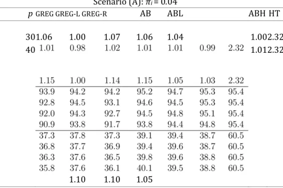
Based on the results, MSEs of AB and GREG are almost the same in all cases since AB is an approximate Bayesian version of GREG. Since AB can take account of the variability in estimating β, the coverage probabilities of AB are closer to the

nominal level (95%) than GREG, which is an important advantage of the proposed method. The GREG shows shorter confidence intervals with large values of p, as the variance estimator is negatively biased, and the coverage rate is lower than the nominal levels. As pgets larger, direct use of the auxiliary information makes the point estimates more inefficient as shown in Table 2, and the methods with shrinkage estimation of β such as ABH, ABL and GREG-L provide better point estimates than AB and GREG, in terms of MSEs. We note that GREG-R does not obtain much gain compared with other shrinkage methods. Comparing ABH, ABL and GREG-L, GREG-L tends to produce short confidence intervals whose coverage probabilities are smaller than the nominal level when pis large, but the proposed ABH and ABL methods produce wider credible intervals than GREG and have coverage probabilities closer to the nominal level.

6.2 Simulationstudy:logisticregression

In the second simulation study, we consider the binary case for yiand apply the

non-linear regression method discussed in Section 5. The binary response variable

Yi∼ Ber(

where β0 = −1 and the other settings are the same as the linear regression case. We again apply the same six methods based on a logistic regression model to obtain point estimates and confidence/credible intervals of the population mean Y¯ =

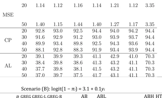
. The obtained MSE, CP and AL based on 1,000 Monte Carlo samples are reported in Table 3, which shows again the superiority of the proposed Bayesian approach to the frequentist approach in terms of uncertainty quantification.

7

Example

We applied the proposed methods to the synthetic income data available from the

sae package (Molina and Marhuenda, 2015) in R language. In the dataset, the

equivalized annual net income is observed for a certain number of individuals in each province of Spain. As auxiliary variables, we used four indicators of the four groupings of ages (16−24, 25−49, 50−64 and ≥ 65 denoted by ag1,...,ag4,

respectively), the indicator of having Spanish nationality na, the indicators of

education levels (primary education ed1 and post-secondary education ed2), and

the indicators of two employment categories (employed em1 and unemployed em2). Moreover, we considered 13 interaction variables; ag1*na, ag2*na, ag3*na,

ag4*na, ag2*ed1, ag3*ed1, ag4*ed1, ag1*em1, ag2*em1, ag3*em1, ag4*em1,

ed1*em1 and ed2*em1. Here we focus on estimating average income in three

provinces, Palencia, Segovia and Soria, where the number of sampled units are 72, 58 and 20, respectively. The number of non-sampled units were around 106_{. In} order to perform joint estimation and inference in the three provinces, we employed the following working model:

  , (26) where belong to province h, where h= 1 for Palencia, h= 2 for

Segovia, and h= 3 for Soria, and xiis the vector of auxiliary variables with dimension

p = 22 (9 auxiliary variables and 13 interaction variables). Here yiis the

log-transformed net income and eiis the error term.

Under the working model (26), the posterior distribution of Y¯his

,

where

,

and

.

Based on the above formulas, we performed the proposed approximate Bayesian methods for Y¯h for each h, and computed 95% credible intervals for the

logtransformed average income with 5000 posterior samples after discarding the first

500 samples as burn-in period. We considered three types of priors for β1, flat,

Laplace and horseshoe priors as considered in Section 6. We also calculated 95% confidence intervals of the log-transformed average income based on the two frequentist methods, GREG and GREG-L, using the working model (26). In applying GREG-L, the tuning parameter in the Lasso estimator was selected via 10 fold cross validation.

The 95% credible intervals of β1 based on the approximate posterior distributions under Laplace and horseshoe priors are shown in Figure 1, in which

the design-consistent and Lasso estimates of β1 are also given. It is observed that

the approximate posterior mean of β1 shrinks the design-consistent estimates of β1 toward 0 although exactly zero estimates are not produced as the frequentist Lasso estimator does. The Lasso estimate selects only one variable among 22 candidates, and the variable is also significant in terms of the credible interval in both two priors. Moreover, the two Bayesian methods detect one or two more variables to be significant judging from the credible intervals. Comparing the results from two priors, the horseshoe prior provides narrower credible intervals than the Laplace prior.

In Figure 2, we show the resulting credible and confidence intervals of the average income in the three provinces. It is observed that the proposed Bayesian methods, AB and ABL, tend to produce wider credible intervals than the confidence intervals of the corresponding frequencies methods, GREG and GREG-L, respectively, which is consistent to the simulation results in Section 6. We can also confirm that the credible intervals of ABH are slightly narrower than those of ABL, which would reflect the differences of interval lengths of β1 as shown in Figure 1.

8

Concluding Remarks

We have proposed an approximate Bayesian method for survey regression estimation using a parametric regression model as the working model. The proposed Bayesian method captures the uncertainty in estimating regression parameters even when the number of the auxiliary variables is large. A main advantage of the proposed method is that it uses a shrinkage prior for regularized regression estimation, which not only provides an efficient point estimator, but also fully captures the uncertainty associated with model selection and parameter estimation via Bayesian inference. Although we only consider two popular prior distributions here, Laplace prior and the horseshoe prior, other priors, such as the

spike-and-slab prior (Ishwaran and Rao, 2005), can be considered. Further investigation regarding the choice of the shrinkage prior distributions will be an important research topic in the future.

Although our working model is parametric, the proposed approximate Bayesian method can be applied to other semiparametric models such as local polynomial model (Breidt and Opsomer, 2000), P-spline regression model (Breidt et al., 2005), or a neural network model (Montanari and Ranalli, 2005). By finding suitable prior distributions for the semiparametric models, the model complexity parameters will be determined automatically and the uncertainty will be captured in the approximate Bayesian framework. Such extensions are beyond the scope of this paper and will be topics for future research.

Acknowledgement

The first author was supported by Japan Society for the Promotion of Science KAKENHI grant number JP18K12757. The second author was supported by US National Science Foundation (MMS-1733572).

Appendix

From (4), we have

Cov

Also, we can show that V(Rn) = O(p/n2) . Therefore, using Chebychev inequality, we

have Rn= Op(p/n) and result (5) follows.

We provide the algorithm for generating the approximate posterior distribution of

β1 given in (20) with two shrinkage priors, Laplace and horseshoe (18) priors. Using the mixture representation of both priors, we get the following Gibbs sampling algorithm.

Laplaceprior

We consider the mixture representation of Laplace distribution: βk|τk∼ N(0,τk2)

and τk2 ∼ Exp(λ2/2), independently, for k= 1,...,p. For λ2, we consider the conjugate

prior Ga(a,b), where Ga(a,b) is a gamma distribution with shape parameter aand rate parameter b. The full conditional distribution of β is multivariate normal with

mean A and variance-covariance matrix A−1 _{where A with D=} diag( ). The full conditional distribution of λ2

is Ga(a+p,b+Ppk=1 τk2/2), and are conditionally independent, with 1/τj2

q 2 _{in the parametrization} conditionally inverse-Gaussian with parameters µ = λ/βjof the inverse-Gaussian

density given by

.

Horseshoeprior

From (18), the prior for β1 can be expressed as a hierarchy: βk|uk∼ N(0,λ2u2k) and

uk∼ HC(0,1) independently for k= 1,...,p, where HC(0,1) is the standard half-Cauchy

distribution. Using the hierarchical expression of the half-Cauchy dis-

tribution, we obtain the following Gibbs sampling steps. Let A , where

B= λ2_{diag( ). The full conditional distribution of β is multivariate normal} with mean A and variance-covariance matrix A−1_{. The full}

  IG and IG ,

where IG(a,b) denotes an inverse-Gamma distribution with shape parameter aand rate parameter b. Here ξk and γ are additional latent variables, and their full

conditional distributions are given by IG(1,1 + 1/δk2) and IG(1,1 + 1/λ2),

respectively.

C.AsketchedproofofTheorem1

To discuss the asymptotic properties of the approximate Bayesian method, we first assume a sequence of finite populations and samples with finite fourth moments as in Isaki and Fuller (1982). The finite population is a random sample from an unknown superpopulation model. Let Y¯∗ and β∗ be the true values of Y¯ and β.

Let Bn= (Y¯∗ −rn,Y¯∗ +rn) and Cnbe a ball with centre β∗ and radius rn∼ nτ−1/2 for 0 < τ

<1/2. We make the following regularity assumptions

(C1) Assume that the sufficient conditions for the asymptotic normality of Yˆ¯reg for

Y¯ ∈ Bnhold for the sequence of finite populations and samples.

(C2) Assume that the prior distribution π(Y¯) is positive and satisfies a Lipschitz condition over its support ΘY; that is, there exists C1 < ∞ such that |π(θ1)− π(θ2)| ≤ C1|θ1 − θ2| for θ1,θ2 ∈ ΘY.

(C3) Assume that Vˆ β = V β{1+oP(1)} and (

β){1 + oP(1)} for any β ∈ Cnand n→ ∞.

Sufficient conditions for (C1) are discussed within various asymptotic structures (e.g. Binder, 1983; Pfeffermann and Sverchkov, 2009). Conditions (C2) and (C4) are satisfied for common priors such as (multivariate) normal distribution . Condition (C3) essentially requires that the design variance estimators be consistent and meet a certain continuity condition.

Proof.Let g(Y,¯ β) = φ(Yˆ¯reg(β);Y,¯ Vˆe(β))φp(βˆ;β,Vˆ β)π(β). Then, the approximated

posterior distribution is given by

.

Note that

(27) By the same argument in the proof of Theorem 1 in Wang et al. (2018), we have

,

so the second term in (27) is oP(1). On the other hand, under condition (C3),

φp(βˆ;β,Vˆ β) = φp(βˆ;β,V β){1+oP(1)} as n→ ∞, for any β ∈ Cn, thereby under

condition (C4),

  Z Z

  g(Y,¯ β)dβ = φ(Yˆ¯reg(β);Y,¯ Vˆe(β))φp(βˆ;β,V β)π(β)dβ

  β∈Cn β∈Cn

= φ(Yˆ¯reg(β∗);Y,¯ Vˆe(β∗))π(β∗){1 + oP(1)}

  (28)   = φ(Yˆ¯reg(βˆ);Y,¯ Vˆe(βˆ)){1 + oP(1)}, (29)

for any Y¯ ∈ Bnas n→ ∞, where (28) follows from (C2), and (29) follows from

the properties Vˆe(βˆ) = Vˆe(β∗){1+oP(1)} and Yˆ¯reg(βˆ) = Y¯ˆreg(β∗){1+oP(1)} under

(C1). Let , where is the

upper β0-quantile of the chi-squared distribution with 1 degree of freedom. Then, plimn→∞ P(Rn) = β0. Since Yˆ¯reg(βˆ) − Y¯∗ = Op(n−1/2) and rn= nτ−1/2, which is slower

than n−1/2_{, it holds that limn→∞ P(Rn⊂ Bn) = 1. Then,}

,

which means that

for any β0 ∈ (0,1), implying

  . (30)

Then,

,

D.AsketchedproofofTheorem2

The condition (C4) given in the proof of Theorem 1 may not be satisfied for shrinkage priors. For example, the horseshoe prior (18) diverge at the origin βk=

0. In what follows, let ) and define βˆ and βˆ(R) _{in the same way. We use} the

following alternative condition for the shrinkage prior πλ(β):

(C5) The regularized estimator βˆRunder penalty −logπλ(β1) is asymptotically

  √ (R)

normal, that is, n(βˆ − β∗) → N(0,C), where Cis a positive definite matrix and λ is appropriately chosen.

Under the Laplace prior, βˆ(R) _{is equivalent to the Lasso estimator, and the above} √

property holds if λ = o( n) (Knight and Fu, 2000; McConville et al., 2017). For general prior πλ(β1), this condition holds if the assumption regarding the penalty term

Pλ(β1) given in Fan and Li (2001) is satisfied.

Proof.It is noted that

Define

g(Y,¯ β) = φ(Yˆ¯reg(β);Y,¯ Vˆe(β))φ(βˆ;β,Vˆ β)πλ(β1).

Z g(Y,¯ β)dβ = φ(Yˆ¯reg(β∗);Y,¯ Vˆe(β∗)){1 + oP(1)} β∈Rn

as n→ ∞, where Rnis a ball with center β∗ and radius O(nτ−1/2) for 0 < τ <1/2. Hence,

the statement can be proved in the same way as the proof of Theorem 1 since φ(Yˆ¯reg(β∗);Y,¯ Vˆe(β∗)) = φ(Yˆ¯reg(βˆ(R));Y,¯ Vˆe(βˆ(R))){1 + oP(1)}.

References

Binder, D. A. (1983). On the variances of asymptotically normal estimators from complex surveys. InternationalStatisticalReviews51, 279–292.

Breidt, F. J., G. Claeskens, and J. D. Opsomer (2005). Model-assisted estimation for complex surveys using penalised splines. Biometrika92, 831–846.

Breidt, F. J. and J. D. Opsomer (2000). Local polynomial regression estimators in survey sampling. AnnalsofStatistics28, 403–427.

Breidt, F. J. and J. D. Opsomer (2017). Model-assisted survey estimation with modern prediction techniques. StatisticalScience32, 190–205.

Carvalho, C. M., N. G. Polson, and J. G. Scott (2009). Handling sparsity via the horseshoe. Proceedings of the 12th International Confe‐ rence on Artificial IntelligenceandStatistics(AISTATS2009).

Carvalho, C. M., N. G. Polson, and J. G. Scott (2010). The horseshoe estimator for sparse signals. Biometrika97, 465–480.

Chen, J. K. T., R. L. Valliant, and M. R. Elliott (2018). Model-assisted calibration of non-probability sample survey data using adaptive LASSO. SurveyMethodology 44, 117–144.

Deville, J. C. and C. E. Sa¨rndal (1992). Calibration estimators in survey sampling.

JournaloftheAmericanStatisticalAssociation87, 376–382.

Fan, J. and R. Li (2001). Variable selection via nonconcave penalized likelihood and its Oracle properties. Journal of the American Statistical Association 96, 1348– 1360.

Fuller, W. A. (2002). Regression estimation for sample surveys. SurveyMethodology 28, 5–23.

Fuller, W. A. (2009). SamplingStatistics. Wiley.

Godambe, V. P. and V. M. Joshi (1965). Admissibility and Bayes estimation in sampling finite populations, 1. AnnalsofMathematicalStatistics36, 1707–1722. Hoerl, E. and R. W. Kennard (1970). Ridge regression: Biased estimation for

nonorthogonal problems. Technometrics12, 55–67.

Horvitz, D. G. and D. J. Thompson (1952). A generalization of sampling without replacement from a finite universe. JournaloftheAmericanStatisticalAssociation 47, 663–685.

Isaki, C. T. and W. A. Fuller (1982). Survey design under the regression superpopulation model. JournaloftheAmericanStatisticalAssociation77, 89–96. Ishwaran, H. and J. S. Rao (2005). Spike and slab variable selection: Frequentist and

Bayesian strategies. AnnalsofStatistics33, 730–773+.

Kim, J. K. and M. Park (2010). Calibration estimation in survey sampling.

InternationalStatisticalReview78, 21–39.

Knight, K. and W. Fu (2000). Asymptotics for Lasso-type estimators. Journal of OfficialStatistics28, 1356–1378.

Little, R. J. A. (2012). Calibrated Bayes, an alternative inferential paradigm for official statistics. JournalofOfficialStatistics.

McConville, K., F. Breidt, T. Lee, and G. Moisen (2017). Model-assisted survey regression estimation with the LASSO. Journal of Survey Statistics and Methodology5, 131–158.

Molina, I. and Y. Marhuenda (2015). sae: An R package for small area estimation.

TheRJournal7, 81–98.

Montanari, G. E. and M. G. Ranalli (2005). Nonparametric model calibration estimation in survey sampling. JournaloftheAmericanStatisticalAssociation100, 1429–1442.

Park, T. and G. Casella (2008). The Bayesian Lasso. Journal of the American StatisticalAssociation103, 681–686.

Pfeffermann, D. and M. Sverchkov (1999). Parametric and semiparametric estimation of regression models fitted to survey data. Sankhy¯a,SeriesB61, 166– 186.

Pfeffermann, D. and M. Sverchkov (2009). Inference under informative sampling.

HandbookofStatistics.

Rao, J. and A. Singh (1997). A ridge-shrinkage method for range-restricted weight calibration in survey sampling. In ProceedingsoftheSectiononSurveyResearch Methods, pp. 57–65. American Statistical Association.

Sa¨rndal, C. E. and Lundstr¨om (2005). Estimationinsurveyswithnonresponse. Chichester: John Wiley & Sons.

Tibshirani, R. (1996). Regression shrinkage and selection via the lasso. Journalof theRoyalStatisticalSociety,SeriesB58, 267–288.

van der Vaart, A. W. (2000). AsymptoticStatistics. New York: Cambridge Uni- versity Press.

Wang, Z., J. K. Kim, and S. Yang (2018). Approximate Bayesian inference under informative sampling. Biometrika105, 91–102.

Wu, C. and R. R. Sitter (2001). A model-calibration approach to using complete auxiliary information from survey data. Journal of the American Statistical Association96, 185–193.

Zou, H. (2006). The adaptive Lasso and its Oracle properties. Journal of the AmericanStatisticalAssociation101, 1418–1429.

Zou, H. and T. Hastie (2005). Regularization and variable selection via the elastic net. JournaloftheRoyalStatisticalSociety,SeriesB67, 301–320.

Table 2: Summary of the simulation results in scenarios (A) and (B) with linear regression. All values are multiplied by 100.

Scenario (A): πi= 0.04

p GREG GREG-L GREG-R AB ABL ABH HT

30 1.06 1.00 1.07 1.06 1.04 1.002.32 40

1.10 1.10 1.05

Scenario (B): logit(1 − πi) = 3.1 + 0.1yi

p GREG GREG-L GREG-R AB ABL ABH HT

  30 1.21 1.12 1.24 1.21 1.24 1.13 3.35   40 1.30 1.13 1.34 1.30 1.25 1.15 3.35

Table 3: Summary of the simulation results in scenarios (A) and (B) with logistic regression. MSE values are multiplied by 10,000 and CP and AL values are multiplied by 100.

Scenario (A): πi= 0.04

p GREG GREG-L GREG-R AB ABL ABH HT

40

3.83 3.78 3.72

3.5512.4

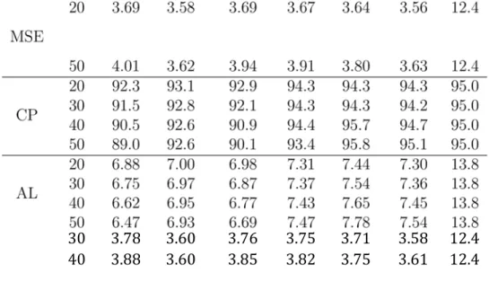
Scenario (B): logit(1 − πi) = 3.1 + 0.1yi

  30 3.78 3.60 3.76 3.75 3.71 3.58 12.4   40 3.88 3.60 3.85 3.82 3.75 3.61 12.4

  Coefficient Coefficient

Figure 1: 95% credible intervals of regression coefficients under Laplace (left) and horseshoe (right) priors.

Figure 2: 95% confidence and credible intervals for average income based on five methods in three provinces in Spain.

Palencia Segovia Soria

GREG AB GREG−L ABL ABH Estimate