Visible Difference Predicator for High Dynamic Range Images

(1)

Visible Difference Predicator for

High Dynamic Range Images

∗

Rafał Mantiuk, Karol Myszkowski, and Hans-Peter Seidel

MPI Informatik, Saarbr¨ucken, Germany

Abstract – Since new imaging and rendering systems com-monly use physically accurate lighting information in the form of High-Dynamic Range data, there is a need for an automatic visual quality assessment of the resulting images. In this work we extend the Visual Difference Predictor (VDP) developed by Daly to handle HDR data. This let us predict if a human observer is able to perceive differences for a pair of HDR images under the adaptation conditions corresponding to the real scene observation.

Keywords: Visual quality metric, high dynamic range, HDR, perception, VDP, contrast sensitivity, CSF, tvi.

1 Introduction

Mainstream imaging and rendering systems commonly use physically accurate lighting information in the form of High-Dynamic Range (HDR) images, textures, environment maps, and light fields in order to capture accurate scene appearance. Unlike their low-dynamic range counterparts, HDR images can describe a full color gamut and entire range of luminance that is visible to a human observer. HDR data can be acquired even with a consumer camera, using multi-exposure techniques [17], which involve taking several pic-tures of different exposures and then combining them to-gether into a single HDR image. Another source of HDR data is realistic image synthesis software, which uses phys-ical values of luminance or radiance to represent generated images. Because HDR images can not be directly displayed on conventional LCD or CRT monitors due to their limited luminance range and gamut, methods of luminance compres-sion (tone mapping) and gamut mapping are required [6]. Even if traditional monitors cannot accurately display HDR data, new displays of extended contrast and maximum lu-minance become available [18, 12]. To limit an additional storage overhead for HDR images, efficient encodings for-mats for HDR images [21, 23, 3, 22] and video [15] have been proposed.

When designing an image synthesis or processing appli-cation, it is desirable to measure the visual quality of the re-sulting images. To avoid tedious subjective tests, where a

∗0-7803-8566-7/04/$20.00 c2004 IEEE.

group of people has to assess the quality degradation, objec-tive visual quality metrics can be used. The most successful objective metrics are based on models of the Human Visual System (HVS) and can predict such effects as a non-linear response to luminance, limited sensitivity to spatial and tem-poral frequencies, and visual masking [16].

Most of the objective quality metrics have been designed to operate on images or video that are to be displayed on CRT or LCD displays. While this assumption seems to be clearly justified in case of low-dynamic range images, it poses prob-lems as new applications that operate on HDR data become more common. A perceptual HDR quality metric could be used for the validation of the aforementioned HDR image and video encodings. Another application may involve steer-ing the computation in a realistic image synthesis algorithm, where the amount of computation devoted to a particular re-gion of the scene would depend on the visibility of potential artifacts.

In this paper we propose several modifications to Daly’s Visual Difference Predicator. The modifications significantly improve a prediction of perceivable differences in the full visible range of luminance. This extends the applicability of the original metric from a comparison of displayed images (compressed luminance) to a comparison of real word scenes of measured luminance (HDR images). The proposed metric does not rely on the global state of eye adaptation to lumi-nance, but rather assumes local adaptation to each fragment of a scene. Such local adaptation is essential for a good pre-diction of contrast visibility in High-Dynamic Range (HDR) images, as a single HDR image can contain both dimly illu-minated interior and strong sunlight. For such situations, the assumption of global adaptation to luminance does not hold. In the following sections we give a brief overview of the objective quality metrics (Section 2), describe our modifica-tions to the VDP (Section 3) and then show results of testing the proposed metric on HDR images (Section 4).

2 Previous work

Several quality metrics for digital images have been pro-posed in the literature [2, 5, 9, 14, 19, 20, 25]. They vary in complexity and in the visual effects they can predict. How-ever, no metric proposed so far was intended to predict

(2)

vis-ible differences in High-Dynamic Range images. If a single metric can potentially predict differences for either very dim or bright light conditions, there is no metric that can process images that contain both very dark and very bright areas.

Two of the most popular metrics that are based on models of the HVS are Daly’s Visual Difference Predicator (VDP) [5] and Sarnoff Visual Discrimination Model [14]. Their predictions were shown to be comparable and the results de-pended on test images, therefore, on average, both metrics performed equally well [13]. We chose the VDP as a base of our HDR quality metric because of its modularity and thus good extensibility.

3 Visual Difference Predicator

In this section we describe our modifications to Daly’s VDP, which enable prediction of the visible differences in High-Dynamic Range images. The major difference between our HDR VDP and Daly’s VDP is that the latter one assumes a global level of adaptation to luminance. In case of VDP for HDR images, we assume that an observer can adapt to every pixel of an image. This makes our predicator more conser-vative but also more reliable when scenes with significant differences of luminance are analyzed. In this paper we give only a brief overview of the VDP and focus on the extension to high-dynamic range images. For detailed description of the VDP, refer to [5].

The data flow diagram of the VDP is shown in Figure 1. The VDP receives a pair of images as an input and gener-ates a map of probability values, which indicgener-ates how the differences between those images are perceived. The first (mask) image of that pair contains an original scene and the second one (target) contains the same scene but with the ar-tifacts whose visibility we want to estimate. The both im-ages should be scaled in the units of luminance. In case of LDR images, pixel values should be inverse gamma cor-rected and calibrated according to the maximum luminance of the display device. In case of HDR images no such pro-cessing is necessary, however luminance should be given in

cd/m2_{. The first two stages of the VDP – amplitude}

com-pensation and CSF filtering (see Figure 1) – compensate for a non-linear response of the human eye to luminance and the loss of sensitivity at high and very low spatial frequencies. Those two stages are heavily modified in our HDR extension and are discussed in Sections 3.1 and 3.2. The next two com-putational blocks – the cortex transform and visual masking – decompose the image into spatial and orientational chan-nels and predict perceivable differences in each channel sep-arately. Since the visual masking does not depend on lumi-nance of a stimuli, this part of the VDP is left unchanged, except for a minor modification in the normalization of units (details in Section 3.3). In the final error pooling stage the probabilities of visible differences are summed up for all channels and a map of detection probabilities is generated. This step is the same in both versions of the VDP.

Amplitude Compression CSF Target Image Mask Image Perceptual Difference Cortex

Transform MaskingVisual

Cortex

Transform MaskingVisual Amplitude

Compression CSF

Error Pooling

Figure 1: Data flow diagram of the Visible Difference Predi-cator (VDP)

3.1 Amplitude Nonlinearity

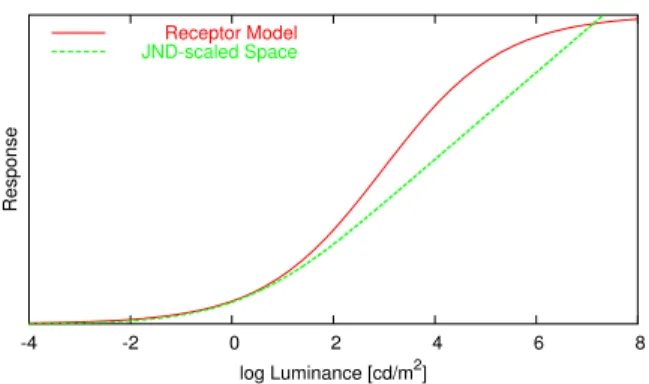
Daly’s VDP utilizes a model of the photoreceptor to ac-count for non-linear response of HVS to luminance. Per-ceivable differences in bright regions of a scene would be overestimated without taking into account this non-linearity. The drawback of using the model of the photoreceptor is that it gives arbitrary units of response, which are loosely related to the threshold values of contrast sensitivity studies. The Contrast Sensitivity Function (CSF), which is responsible for the normalization of contrast values to JND units in Daly’s VDP, is scaled in physical units of luminance. Therefore us-ing a physical threshold contrast to normalize response val-ues of the photoreceptor may give an inaccurate estimate of the visibility threshold. Note that the response values are non-linearly related to luminance. Moreover, the model of photoreceptor, which is modeled as a sigmoidal function (see Figure 2), assumes equal loss of sensitivity for low and high luminance levels, while it is known that loss of sensitivity is observed only for low luminance levels (see Figure 3). Even if the above simplifications are acceptable for low-dynamic range images, they may lead to significant inaccuracies in case of HDR data.

Instead of modeling the photoreceptor we propose con-verting luminance values to a non-linear space that is scaled in JND units [1, 15]. Such space should have the following

property: Adding or subtracting a value of1in this space

results in a just perceivable change of relative contrast. To find a proper transformation from luminance to such JND-scaled space, we follow a similar approach as in [15]. Let the threshold contrast be given by thethreshold versus intensity

(tvi) function [10]. Ify = ψ(l)is a function that converts values in JND-scaled space to luminance, we can rewrite our property as:

ψ(l+ 1)−ψ(l) =tvi(yadapt) (1) wheretviis athreshold versus intensityfunction andyadapt

is adaptation luminance. A value of the tvifunction is a

minimum difference of luminance that is visible to a human observer. From the first-order Taylor series expansion of the above equation, we get:

dψ(l)

dl =tvi(yadapt) (2)

Assuming that the eye can adapt to a single pixel of lumi-nanceyas in [5], that isyadapt=y=ψ(l), the equation can

(3)

be rewritten as:

dψ(l)

dl =tvi(ψ(l)) (3)

Finally, the functionψ(l)can be found by solving the above

differential equation. In the VDP for HDR images we have to find a value oflfor each pixel of luminancey, thus we do not need functionψ, but its inverseψ−1. This can be easily

found since the functionψis strictly monotonic.

The inverse functionl = ψ−1(y) is plotted in Figure 2

together with the original model of photoreceptor. The func-tion properly simulates loss of sensitivity for scotopic levels of luminance (compare with Figure 3). For the photopic lu-minance, the function has logarithmic response, which cor-responds to Weber’s law. Ashikhmin [1] derived a similar

function for the tone mapping purpose and called it the

ca-pacity function.

The actual shape of the threshold versus intensity (tvi) function has been extensively studied and several models have been proposed [8, 4]. To be consistent with Daly’s

VDP, we derive atvifunction from the CSF used there. We

find values of thetvifunction for each adaptation luminance yadaptby looking for the peak sensitivity of the CSF at each yadapt:

tvi(yadapt) =P·

yadapt maxρCSF(ρ, yadapt)

(4)

whereρdenotes spatial frequency. Similar as in the Daly’s

VDP, parameter P is used to adjust the absolute peak thresh-old. We adjusted the value of P in our implementation, so that the minimum relative contrast is 1% – a commonly as-sumed visibility threshold [10, Section 3.2.1]. A function of relative contrast –contrast versus intensitycvi=tvi/yadapt – is often used instead oftvifor a better data presentation. Thecvifunction for our derivedtviis plotted in Figure 3.

In our HDR VDP we use a numerical solution of Equa-tion 3 and a binary search on this discrete soluEqua-tion to convert

luminance valuesytolin JND-scaled space. The subsequent

parts of the HDR VDP operate onlvalues.

3.2 Contrast Sensitivity Function

The Contrast Sensitivity Function (CSF) describes loss of sensitivity of the eye as a function of spatial frequency and adaptation luminance. It was used in the previous section to

derive thetvifunction. In Daly’s VDP, the CSF is

respon-sible for both modeling loss of sensitivity and normalizing contrast to JND units. In our HDR VDP, normalization to units of JND at the CSF filtering stage is no longer neces-sary as the non-linearity step has already scaled an image to JND units (refer to the previous section). Therefore the CSF should predict only loss of sensitivity for low and high spa-tial frequencies. Loss of sensitivity in JND-scaled space can be modeled by a CSF that is normalized by peak sensitivity for particular adaptation luminance:

CSFnorm(ρ, yadapt) = CSF(ρ, yadapt) maxρCSF(ρ, yadapt) (5) -4 -2 0 2 4 6 8 Response log Luminance [cd/m2] Receptor Model JND-scaled Space

Figure 2: Response curve of the receptor model used in Daly’s VDP (red) and mapping to JND-scaled space used in our HDR extension of the VDP (green). The sigmoidal re-sponse of Daly’s receptor model (adaptation to a single pixel)

overestimates contrast at luminance levels above10cd/m2

and compresses contrast above10000cd/m2_.

Psychophys-ical findings do not confirm such luminance compression at high levels of luminance. Another drawback of the recep-tor model is that the response is not scaled in JND units, so that CSF must be responsible for proper scaling of luminance contrast.

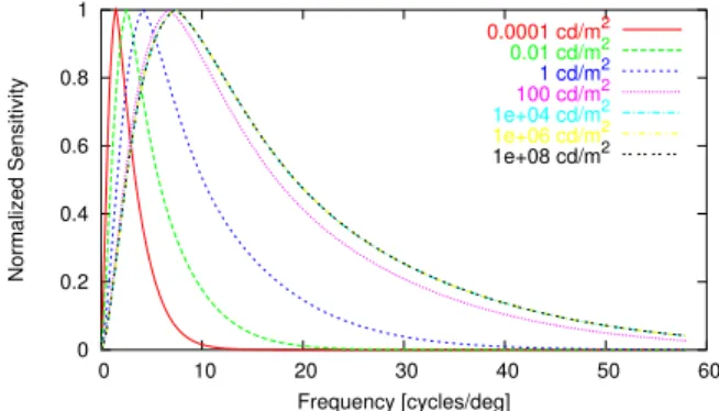
Unfortunately, in case of HDR images, a single CSF can not be used for filtering an entire image since the shape of the CSF significantly changes with adaptation luminance.

The peak sensitivity shifts from about2 cycles/degreeto

7cycles/degreeas adaptation luminance changes from

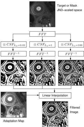
sco-topic to phosco-topic, see Figure 4. To account for this, to filter an image, a separate convolution kernel should be used for each pixel. Because the support of such convolution kernel can be rather large, we use a computationally more effec-tive approach in our implementation of the VDP for HDR images: We filter an image in FFT space several times, each time using CSF for different adaptation luminance. Then, we convert all the filtered images to the spatial domain and use them to linearly interpolate pixel values. We use luminance values from the original image to determine the adaptation luminance for each pixel (assuming adaptation to a single pixel) and thus to choose filtered images that should be used for interpolation. A more accurate approach would be to compute the adaptation map [24], which would consider the fact that the eye can not adapt to a single pixel. A similar approach to non-linear filtering, in case of a bilateral filter, was proposed in [7]. The process of filtering using multiple CSFs is shown in Figure 5.

As can be seen in Figure 4, the CSF changes its shape significantly for scotopic and mesopic adaptation luminance and remains constant above1000cd/m2_{. Therefore it is}

usu-ally enough to filter the image using a CSF for yadapt =

{0.0001,0.01, ...,1000}cd/m2_{. The number of filters can}

be further limited if the image has a lower range of lumi-nance.

(4)

0.001 0.01 0.1 1 -4 -2 0 2 4 6 8 Threshold Contrast log Luminance [cd/m2]

Contrast Versus Intensity

Figure 3:Contrast versus intensitycvifunction predicts the

minimum distinguishable contrast at a particular adaptation level. It is also a conservative estimate of a contrast that in-troduces a Just Noticeable Difference (JND). The higher val-ues of thecvifunction at low luminance levels indicate loss of sensitivity of the human eye for low light conditions. The

cvicurve shown in this figure was used to derive a function

that maps luminance to JND-scaled space.

3.3 Other Modifications

An important difference between Daly’s VDP and the pro-posed extension for HDR images is that the first one oper-ates on CSF normalized values and the latter one represents channel data in JND-scaled space. Therefore, in case of the VDP for HDR images, original and distorted images can be compared without any additional normalization and scaling. This is possible because a difference between the images that equals one unit in JND-scaled space gives a probability of detection equal to one JND, which is exactly what this step of the VDP assumes. Therefore the contrast difference in Daly’s VDP: ∆Ck,l(i, j) = B1k,l(i, j) BK −B2k,l(i, j) BK (6) in case of the VDP for HDR images becomes:

∆Ck,l(i, j) =B1k,l(i, j)−B2k,l(i, j) (7)

where k, l are channel indices, i, j pixel coordinates and

B1, B2are corresponding channel values for the target and

mask images.

4 Results

To test how our modifications for HDR images affected a prediction of the visible differences, we compared the results of Daly’s VDP and our modified HDR VDP.

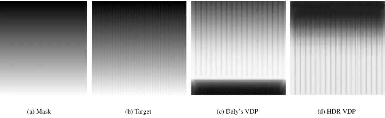
The first pair of images contained a luminance ramp and the same ramp distorted by a sinusoidal grating (see Fig-ure 6). The probability map of Daly’s VDP (FigFig-ure 6(c)) shows lack of visible differences for high luminance area (bottom of the image). This is due to the luminance compres-sion of the photoreceptor model (compare with Figure 2).

0 0.2 0.4 0.6 0.8 1 0 10 20 30 40 50 60 Normalized Sensitivity Frequency [cycles/deg] 0.0001 cd/m2 0.01 cd/m2 1 cd/m2 100 cd/m2 1e+04 cd/m2 1e+06 cd/m2 1e+08 cd/m2

Figure 4: Family of normalized Contrast Sensitivity Func-tions (CSF) for different adaptation levels. The peak sensi-tivity shifts towards lower frequencies as the luminance of adaptation decreases. Shape of the CSF does not change

sig-nificantly for adaptation luminance above 1000cd/m2_.

The HDR VDP does not predict loss of visibility for high lu-minance (Figure 6(d)), but it does for lower lulu-minance levels, which is in agreement with thecontrast versus intensity char-acteristic of the HVS. The visibility threshold for average and low luminance is also lowered by the CSF, which

sup-presses the grating of5cycles/degreefor luminance lower

than1cd/m2_{(see Figure 4). Because Daly’s VDP filters}

im-ages using the CSF for a single adaptation level, there is no difference in the grating suppression for both low and high luminance regions of the image.

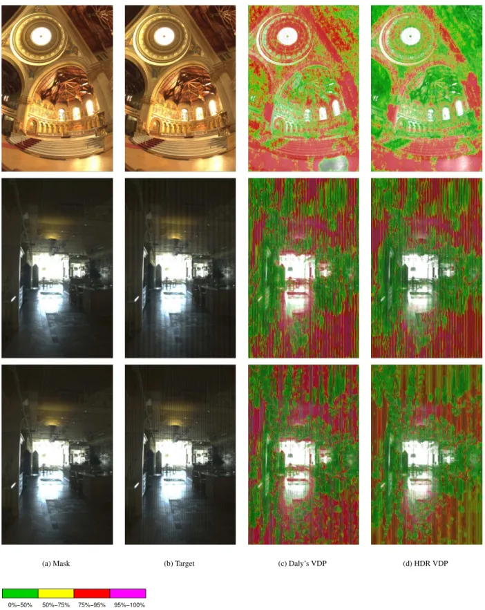
The next set of experiments was performed on HDR im-ages, which are commonly used for testing tone mapping operators. The first row of Figure 7 shows a prediction of

contouring artifacts in the Memorial Churchimage. Both

VDPs predicted properly visibility of the artifacts in the non-masked areas (floor and columns). However, Daly’s VDP failed to predict distortions in the bright highlight on the floor (bottom right of the image), which can be caused by exces-sive luminance compression at high luminance levels. Daly’s metric also overestimated visible differences in dark regions

of the scene. Similar results were obtained for theDesign

Centerimage distorted by a sinusoidal grating of different frequencies (the second and third row of Figure 7). High frequency noise (the third row) was suppressed for the low luminance region of the image (the right bottom corner) only in case of the HDR VDP. Such noise is mostly visible in the brighter parts of the image – the ceiling lamp and the areas near the window – for which the CSF predicts higher sensi-tivity at high frequencies.

More tests should be performed in the future to test the prediction of masking. The validation done in this work con-firmed a better prediction of HDR VDP at high luminance levels (in accordance with thecvi) and at low luminance lev-els in the presence of high frequency patterns (in accordance with the CSF).

(5)

(a) Mask (b) Target (c) Daly’s VDP (d) HDR VDP

Figure 6: A logarithmic luminance ramp (a) from10−4cd/m2(top of the image) to106cd/m2(bottom of the image) was

distorted with a sinusoidal grating of contrast 10% and frequency5cycles/degree(b). The original and the distorted image

was compared using both versions of the VDP and the resulting probability map was shown in subfigures c and d, where brighter gray-levels denote higher probability.

5 Conclusion

In this paper we derive several extensions to Daly’s Visual Difference Predicator from psychophysical data. The exten-sions enable the comparison of High-Dynamic Range im-ages. The proposed JND-scaled space is used to predict a just noticeable differences at luminance adaptation levels rang-ing from dark scotopic to extremely bright photopic. The extended CSF filtering stage can predict loss of sensitivity for high frequency patterns at scotopic conditions and at the same time high sensitivity for those patterns in bright parts of the image. We also verified integrity of the HDR VDP and made adjustments, where differences to Daly’s VDP were caused by using different units to represent contrast.

In future work we would like to further extend the VDP to handle color images in a similar way as it was done in [11], but also take into consideration extended color gamut. A more extensive validation of HDR VDP predictions, possibly using a HDR display, is necessary to confirm good correla-tion between the predicted distorcorrela-tions and the actual quality degradation as perceived by a human observer.

Acknowledgments

We would like to thank Scott Daly for his stimulating com-ments on this work. We would also like to thank Gernot Ziegler for proofreading the final version of this paper.

References

[1] M. Ashikhmin. A tone mapping algorithm for high

contrast images. InRendering Techniques 2002: 13th

Eurographics Workshop on Rendering, pages 145–156, 2002.

[2] P. Barten. Subjective image quality of high-definition television pictures. InProc. of the Soc. for Inf. Disp., volume 31, pages 239–243, 1990.

[3] R. Bogart, F. Kainz, and D. Hess. OpenEXR image file

format. InACM SIGGRAPH 2003, Sketches &

Appli-cations, 2003.

[4] CIE. An Analytical Model for Describing the

Influ-ence of Lighting Parameters Upon Visual Performance, volume 1. Technical Foundations, CIE 19/2.1. Interna-tional Organization for Standardization, 1981. [5] S. Daly. The Visible Differences Predictor: An

algo-rithm for the assessment of image fidelity. In A.

Wat-son, editor, Digital Image and Human Vision, pages

179–206. Cambridge, MA: MIT Press, 1993.

[6] K. Devlin, A. Chalmers, A. Wilkie, and W. Purgathofer. Tone Reproduction and Physically Based Spectral Ren-dering. InEurographics 2002: State of the Art Reports, pages 101–123. Eurographics, 2002.

[7] F. Durand and J. Dorsey. Fast bilateral filtering for the

display of high-dynamic-range images. InProceedings

of the 29th annual conference on Computer graphics and interactive techniques, pages 257–266, 2002. [8] J. Ferwerda, S. Pattanaik, P. Shirley, and D.

Green-berg. A model of visual adaptation for realistic

im-age synthesis. InProceedings of SIGGRAPH 96,

Com-puter Graphics Proceedings, Annual Conference Se-ries, pages 249–258, Aug. 1996.

[9] D. Heeger and P. Teo. A model of perceptual image

fidelity. InProc. of IEEE Int’l Conference Image

Pro-cessing, pages 343–345, 1995.

[10] D. Hood and M. Finkelstein. Sensitivity to light. In

K. Boff, L. Kaufman, and J. Thomas, editors,

Hand-book of Perception and Human Performance: 1. Sen-sory Processes and Perception, volume 1, New York, 1986. Wiley.

(6)

Adaptation Map Filtered Image Target or Mask JND−scaled space Linear Interpolation F F T−1 F F T−1 _{F F T}₋1 F F T ⊗CSF_La=0_.01 ⊗CSF_La=1 ⊗CSFLa=100

Figure 5: To account for a changing shape of the Contrast Sensitivity Function (CSF) with luminance of adaptation, an image is filtered using several shapes of CSF and then the fil-tered images are linearly interpolated. The adaptation map is used to decide which pair of filtered images should be chosen for the interpolation.

[11] E. W. Jin, X.-F. Feng, and J. Newell. The development of a color visual difference model (CVDM). InIS&T’s 1998 Image Processing, Image Quality, Image Capture, Systems Conf., pages 154–158, 1998.

[12] P. Ledda, G. Ward, and A. Chalmers. A wide field, high

dynamic range, stereographic viewer. InGRAPHITE

2003, pages 237–244, 2003.

[13] B. Li, G. Meyer, and R. Klassen. A comparison of two

image quality models. InHuman Vision and Electronic

Imaging III, pages 98–109. SPIE Vol. 3299, 1998. [14] J. Lubin. A visual discrimination model for imaging

system design and evaluation. InVis. Models for Target Detection, pages 245–283, 1995.

[15] R. Mantiuk, G. Krawczyk, K. Myszkowski, and H.-P. Seidel. Perception-motivated high dynamic range

video encoding. ACM Transactions on Graphics,

23(3):730–738, 2004.

[16] M. Nadenau. Integration of Human color vision

Mod-els into High Quality Image Compression. PhD thesis, École Polytechnique Fédéral Lausane, 2000.

[17] M. Robertson, S. Borman, and R. Stevenson. Dy-namic range improvement through multiple exposures. InProceedings of the 1999 International Conference on Image Processing (ICIP-99), pages 159–163, Los Alamitos, CA, Oct. 24–28 1999.

[18] H. Seetzen, W. Heidrich, W. Stuerzlinger, G. Ward, L. Whitehead, M. Trentacoste, A. Ghosh, and A. Vorozcovs. High dynamic range display systems.

ACM Transactions on Graphics, 23(3):757–765, 2004. [19] C. Taylor, Z. Pizlo, J. P. Allebach, and C. Bouman. Im-age quality assessment with a Gabor pyramid model

of the Human Visual System. InHum. Vis. and Elect.

Imaging, pages 58–69. SPIE Vol. 3016, 1997.

[20] Z. Wang and A. Bovik. A universal image quality

index. IEEE Signal Processing Letters, 9(3):81–84,

2002.

[21] G. Ward. Real pixels.Graphics Gems II, pages 80–83,

1991.

[22] G. Ward and M. Simmons. Subband encoding of high

dynamic range imagery. InProceedings of the 1st

Sym-posium on Applied Perception in Graphics and Visual-ization, 2004.

[23] G. Ward Larson. Logluv encoding for full-gamut,

high-dynamic range images. Journal of Graphics Tools,