CHAPTER 47 THE GENERATION OF LONG WAVES IN THE LABORATORY INTRODUCTION

THE GENERATION OF LONG WAVES IN THE LABORATORY by Derek Goring1 and Fredric Raichlen2

INTRODUCTION

It became evident in the experimental aspects of a recent study of the propagation of nonlinear long waves past a step and up a slope that it was important to be able to generate waves which were initially well defined. The investigation dealt with the reflection and transmission of tsunamis past the continental shelf-break, and as such, two simple waves were used to represent certain characteristics of tsunamis: solitary waves and cnoidal waves. (Both of these permanent waves are solutions to the Korteweg-de Vries equation which to a certain order describe the propagation in two dimensions of nonlinear dispersive shallow water waves (see, e.g. Whitham, 1974).)

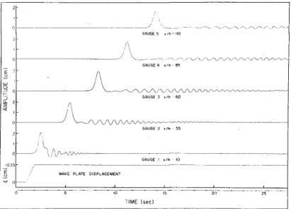
The solitary wave actually can be generated in the laboratory in a simple manner if the wave tank is long enough and wave groups trailing the main wave are unimportant to the study. An example of the resulting waves obtained in the laboratory using a crude generation, procedure is demonstrated by the oscillograph record presented in Figure 1. Six traces are shown: the one at the bottom of the figure describes the time-displacement history of a vertical bulkhead wave generator which is moved by a hydraulic-servo system, the other five are the time variations of the water surface obtained using resistance wave gages spaced at the indicated number of depths downstream from the generator. (In the example presented, the depth of water was 10 cm and the wave plate was moved linearly with time a distance of 10.33 cm in 0.8 sec.) The wave gener- ated and first shown 10 depths downstream appears to qonsist of a large wave followed by a series of oscillatory waves (termed the tail). As would be expected, as the waves propagate, due to the frequency content and the amplitude of the waves, the system separates into a leading wave followed some distance behind by the tail. The lead wave has the charac- teristic shape of a solitary wave. However, if the oscillatory tail is unacceptable for the type of experiments being conducted, and if it cannot be eliminated or the method of elimination is unacceptable, then a means of generation must be sought which eliminates the trailing waves initially.

The method used in this study to produce a nonlinear shallow water wave which is well formed near the generator attempts to match the velocities of the wave plate and the water particles of the desired wave as the plate moves. An example of the result of doing this for a solitary wave is shown in the oscillograph record presented in Figure 2; again the motion of the wave generator is shown at the bottom of the 'Scientist, Christchurch Science Centre, New Zealand Ministry of Works &

Development; formerly Grad. Student, W, M. Keck Lab of Hydr. & Water Res., California Institute of Technology, Pasadena, CA.

2Professor of Civil Engineering, W. M. Keck Lab of Hydr. & Water Res., California Institute of Technology, Pasadena, CA.

H °

4 2

GAUGE 5 x/h = 110

/ WAVE PLATE DISPLACEMENT

GAUGE 2 x/tt - 35

GAUGE I x/h = 10

Figure 1 Oscillograph record of the waves generated by a ramp trajectory (S = 10.33 cm, T = 0.80 sec and h = 10 cm).

2 0 2

-

J\

-

A

°

-

_A

<

__A___

'\

/

vj o

,

,

0 5 10 TIME (sec)

15 20

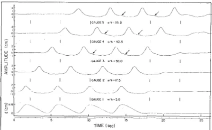
Figure 2 Oscillograph record of the waves generated by the solitary wave trajectory with H/h = 0.2 (S = 10.33 cm, x = 2.044 sec and h = 10 cm).

figure and five wave profiles are presented above. (The location of the wave gages are the same as in Figure 1.) The motion (or trajectory) of the wave plate is no longer linear and the time of motion is more than twice that for the case shown in Figure 1, i.e., x = 2.044 sec. A comparison of the time history of the water surface elevation at 110 depths downstream of the generator shows the trailing oscillatory waves essentially have been eliminated.

Similar time histories of water surface and wave generator displace- ments are presented in Figures 3 and 4 for periodic wave plate motions.

(It was desired for this example to produce cnoidal waves which, as mentioned, are the exact periodic solution of the Korteweg-de Vries equation.) Figure 3 shows the wave resulting from an "incorrect" plate motion where the shape changes as it propagates; note the period of the plate motion is T = 4.28 sec. When the same trajectory is used but a "correct" period is chosen (T = 2.90 sec) a system of waves is generated with the central portion of the train appears relatively unchanged for the nearly 60 depths of propagation shown. The shape of these waves and their method of generation will be discussed more fully later; suffice to say that Figures 2 and 4 demonstrate, at least qualitatively, that the desired system of waves can be generated if adequate attention is given to the method of generation.

ANALYTICAL CONSIDERATIONS

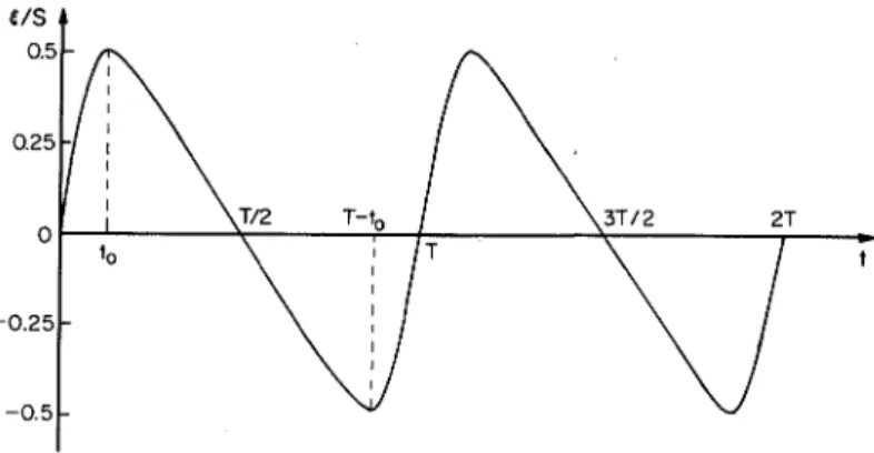
A qualitative description of the generation process is provided by the phase-plane presented in Figure 5. The upper part of the figure (Part c) shows a desired sinusoidal water surface profile; in the lower left the corresponding horizontal water particle velocity time history is given. (For purposes of this discussion it is assumed the water particle

(V) (c)

/;-x

TIME (sec)

Figure 3 Oscillograph record showing the waves generated by tra- jectory CN4 with h = 20 cm, S = 11.18 cm and T = 4.28 sec.

E z LJ Q £ 11.18 GAUGES x/h«l7.5 GAUGE I x/h=5.0

/\. WAVE PLATE DISPLACEMENT

TIME (sec)

Figure 4 Oscillograph record showing the waves generated by tra- jectory CN4 with h = 20 cm, S = 11.18 cm and T = 2.90 sec.

velocity distribution is either constant with depth or that represented in Figure 5 a is the depth-averaged velocity.) If in the x-t plane (Part b) the wave propagates unchanging to the right with celerity c, the wave properties such as amplitude and velocity propagate along lines which are straight and parallel and have a slope dx/dt = c. The time-history of the motion of the wave plate which generated the wave is represented in Part b by the curve £(t) which is termed the "trajectory" in this study.

Referring to Figure 5-j for time t.< 0 the wave plate is at rest and 5=0. At time t = 0 the wave plate begins to move along the trajectory 5(t). The object of this development is to determine the trajectory £(t) which will generate a given long wave n(x,t) with permanent shape propa- gating with celerity c. As mentioned previously, the basic concept is to match the velocity of the wave plate, dg/dt, at all positions, with the corresponding velocity of the water particles (or the depth-averaged velocity) under the long wave, i.e., TT(x,t). Thus, on the face of the wave maker:

&"u(C,t) (1)

Including the position of the plate, 5, in the velocity, u"(g,t), takes Into account that during the generation process the wave is propagating away from the plate. The effect is to produce a trajectory which is dis- torted from what 1t would be if the velocity at the mean position of the plate, u(0,t) were used. This can be seen in Figure 5, where if the velocity u(0,t) were used in Eq. (1), the trajectory would be sinusoidal and the maximum displacement of the plate, 5 = S, would occur at time %T. However, Figure 5(b) shows that the maximum of the trajectory occurs at t = %T +S/c. Thus, the time taken for the plate to travel to its maxi- mum position is S/c longer than it would be if a sinusoidal trajectory were assumed, and consequently the time for the plate to travel back to its original position is time S/c shorter than for a sinusoidal trajec- tory. Therefore, the effect of including the position £ in the velocity is that when the plate and wave are moving in the same direction, the time coordinate stretches; when the plate and the wave are moving in opposite directions, the time coordinate contracts.

The simple sinusoidal variation of the water particle velocity shown in Figure 5a was presented as an example; for finite amplitude shallow water waves of permanent shape it can be shown from continuity considerations that the velocity averaged over the depth is:

TjYx t) = c n(x»*) (?)

UlX,t' h+n(x,t) • (2)

where h is the depth, and n(x,t) and c are defined in Figure 5. Thus, in terms of the plate velocity, from.Eq. (1):

d£= c ri(5,t)

dt h+n(5,t) (3)

Eq. (3) must be integrated to obtain the trajectory, £(t). It is assumed that at the position of the wave plate the wave has the form:

l~~ ct ~ &>

n(5.t) = H[f(e)3 , (4)

where ,., £ 9 = k(ct - 5) . (5) - 4- U- By algebraic manipulation of Eqs. (3), (4) and (5) it can be shown that: v-

and de €f(e)] kh 8 5(t) • = i/fMdw •ID (7) where w is the dummy variable of integration. Equation (7) is an implicit equation which in general, for a particular time t, must be solved numerically. The most efficient method of solution was found to be Newton's Rule. Using Eq. (5), 6 is substituted for the displacement 5

in Eq. (7) to yield: e

F = 6 - kct + £ /f (w)dw = 0 . (8) "o

Equation (8) must be solved for 9 at a given time t. Differentiating Eq. (8):

Newton's Rule is:

ff=n-{ifCe) ,

(9)

^>.

H>.r(e

;i) , (10)

F

(ev")

where superscripts denote iteration number and Ffi = 3F/88. Substituting

for F and FQ in Eq. (10) yields: H ^j

,(1+1) . „(D 1

(i)-kct + JL / f(w)dw

f f(w)

i+ftf{elr')

OD

5 = ct - e/k . (12)

Eqs. (7), or (11) and (12) provide the wave plate displacement as a function of time, 5(t), for a general wave form f(9). These equations will now be applied for specific functions f(e) which describe solitary and cnoidal waves. For a solitary wave which satisfies the Korteweg- de Vries equation, the wave function f(6) in Eq. (4) is:

where e-K(ct-s), K = \/fjjir > c =yjg(\\+H),

Substituting Eq. (13) into the generation equation, Eq. (7), and per- forming the integration yields:

e(t)

In Figure 6 a typical trajectory, 5(t), is presented which was calcu- lated from Eq. (14). The origin of the displacement £ and of the time t occurs at the wave crest in accordance with the definition of the soli- tary wave, Eq. (13). In addition, since the function f(6) in Eq. (13)

c^^^^^JJ-

cJ

Figure 6 Phase plane showing typical wave plate trajectory for a solitary wave.

tends to zero as 6 goes to infinity, the intercepts of the characteris- tics associated with the leading and trailing edges of the wave with the time axis, ± t0, occur at ± » . However, for practical purposes, to three significant figures, the intercept, t0, may be defined as:

t _ tanh~'(0.999)

O ~ KC

The stroke S is obtained by evaluating Eq. t = - oo and subtracting to yield:

3.80

KC (15)

(14) at.time t = + °° and

_ 2H _

fTF"

The duration of motion T is obtained (see Figure 6) by computing the times at which the leading and trailing edge characteristics intersect the trajectory £(t) and subtracting; thus:

2to + S/c . (17)

•» and ₀ stroke S yields for the duration:

ice V 5.80 + jj-' )• (18)

(In practice, the origin of the trajectory, 5(0), is moved to the point ( - x/2, - S/2) in the x-t plane so that motion starts from rest and proceeds in the forward direction.)

Substituting Eqs. (15), (16) and (18) in Eq. (14) and rearranging gives the following normalized form of the generation equation for

solitary waves: / ^ _r>

|4{l

tanh

[(3.80 4)(i4)-K(|.l)]

. (Jg) '

A family of normalized generation trajectories calculated using Eq. (1 is presented in Figure 7 for wave height-to-depth ratios of H/h = 0.1 ;nted in Figure 7 for wave heiqht-to-depth ratios of H/h = 0 (14) to 0.7.

The Korteweg-de Vries equation has a solution which is a permanent form periodic wave usually termed the cnoidal wave. Using the general form shown in Eq. 4 for cnoidal waves the function f(6) is:

f(e) = -\- + cn2(9|m) , (20)

where 6 = 2I<( y - f-\ and K is the first complete elliptic integral, en is the Jacobian elliptic function, m is the elliptic parameter, T is the period, L is the wave length, yt is the distance from the bottom to the trough of the wave, and h is the depth. Substituting Eq. (20) into the generation equation, Eq. (7), and performing the integration yields:

5(t) =

2Kh {

t"

m[

l

"

'

]} •

where E(e|m) is the second incomplete elliptic integral, and m' is the

complementary parameter, m1 = 1 - m.

In Figure 8 a typical trajectory, ?(t), is presented which is normalized with respect to the total movement (stroke) of the wave

plate, 5max = S/2, calculated from Eq. (21). Because of the definition

of the function f(8) in Eq. (20), the origin occurs at a point of maxi- mum velocity. However, it is desirable to start the motion of the wave plate at a position where the velocity of the plate and the amplitude

f/S 0.5 0.25 0 \T/2 T-t„ \3T/2 2T to J t 0.25

-

Figure 8 Typical wave plate trajectory for cnoidal wave generation, of the wave are each zero, i.e., where:,

17=0 , (22)

dt

and

n

0

The parameter 60 is the argument of the cnoidal function determined such

that the wave amplitude is zero. Eq. (23) can be written as:

1/2

ra •

Substituting for 6 in Eq. (21) realizing this is the position of maximum plate displacement gives:

Tiiax Tnl

n--m{(yt-*\

n[^oW-

\]}

W

and

t £6 _{o _ ^max , o}

1 — +

L 2K -

The maximum excursion of the wave plate (or stroke S) is: S = 25mfl¥ .

(26)

(27) Since the leading wave of a group of cnoidal waves would be a transient wave, it was desirableto make this wave a positive wave rather than a negative wave so the train would not overtake it. Thus, the motion is started at a minimum-point in Figure 8, i.e., the origin of the trajec- tory is at t = T - t0. (The interested reader is referred to Goring

(1978) for details of the numerical procedures involved in defining the cnoidal wave relationships.)

Six trajectories for cnoidal waves which were used in this study are presented in Figure 9 (denoted as CN1 to CN6) along with the corres- ponding profiles of the waves the theory predicts will be generated. In theory each cnoidal wave is defined by the parameters: H/h and T/g/h which are shown next to each wave in the table to the right in Figure 9. However, for a given value of t /T it has been found that reasonably good cnoidal waves can be produced with the appropriate pairs of H/h and T/g/h (see Goring, 1978).

Certain other characteristics of the generation process will be discussed later when the theoretical results are compared to the results of experiments.

EXPERIMENTAL EQUIPMENT AND PROCEDURES

The wave generator used in this study consists of a vertical plate which is moved horizontally in a prescribed manner by means of an electro- hydraulic servo-system which is driven by a programmed input voltage. The displacement-time history of the wave-plate is directly proportional to the time history of the input voltage.

In general, the system is similar to many other hydraulically operated wave machines in use; hence, only one unique aspect will be discussed here. That is the function generator which provides a voltage- time history which is proportional to the desired trajectory of the wave plate (as was shown schematically in Figure 5). The function generator used in this investigation consists of a device which is capable of storing 1000 three digit words. The memory can be filled either manually or through a punched paper tape reader; the data rate and the voltage of the output can be changed over a wide range. In this way, for a given shape of the trajectory, the amplitude and the duration of the motion can be adjusted.

The wave tank in which the piston type wave generator is mounted is 37.7 m long, 61 cm deep, and 39.4 cm wide. The tank is constructed of 13 modules each of which has been leveled accurately. The bottom is com- posed of sections of structural steel channel and the sidewalls are glass throughout.

All wave profile measurements were made using resistance wave gages whose sensitive elements were two parallel stainless steel wires (0.25 mm dia.) spaced 4 mm apart. The wires were stretched taut in a "C" shaped frame of stainless steel rod. These gages were used in conjunc- tion with a Hewlett Packard (7700 Series) oscillograph for most measure- ments. Some detailed profiles were obtained with the aid of an analog- to-digital converter so that data reduction and plotting were accomplished using a digital computer.

PRESENTATION AND DISCUSSION OF RESULTS

As noted in Figure 1, if a linear trajectory of the wave machine were used to generate a solitary wave, for the conditions shown an

o o' d

I

\

\

o

d <0 io o

o d

o

(/)

>>

*

oscillatory tail with waves about 25% of the height of the leading wave would be present. As a better approximation, if the generation equations were solved assuming small motions of the generator the height of the waves in the tail could be reduced to about 10% of the first wave. Using the full theory for solitary wave generation (Eq. 19) results in the wave profiles presented in Figure 2, which shows that oscillatory waves nearly can be eliminated by a correct wave generation program. For the waves shown in Figure 2 the duration is x = 2.044 sec which is 7.4% greater than that predicted by Eq. (18); this difference decreases the magnitude of the trailing waves. That the optimum duration is not the theoretical duration is due in part to the fact that the wave plate velocity is constant with depth whereas there 1s a variation of hori- zontal water particle velocity with depth under a solitary wave. Thus, the desired boundary condition is not met precisely at the wave plate for this type of generator.

A comparison of experimentally determined profiles of solitary wayes with two theories is presented in Figure 10. The theories chosen for comparison are those developed by Boussinesq (1782) and McCowan (1891) and the appropriate expressions for the profiles are shown in Table 1.

Table 1 Solutions of the solitary wave due to Boussinesq (1782j and McCowan (1891).

Boussinesq McCowan

Wave profile ri =

_H-*

₂

_Vff

MIcosMa+n/h) +coshM^j Wave speed C = r M /gh(l+H/h) Note N and M are:

» = !

si

4

M

H!)]

In Figure 10 waves with ratios of height to depth of 0.15 and 0.61 are shown and in both cases the agreement with each of the two theories is reasonable. The smaller wave agrees well with the Boussinesq theory over nearly the full range of the abscissa. The same degree of agree- ment is not apparent for the larger wave; however, over the major

0.16 0.12 - 0.8 - 0.4

, ,,., ,

-

/

"*\

~

-

Figure 10 Comparison of the shape of solitary waves with relative heights (a) H/h = 0.15 and (b) H/h = 0.61 with the theories of

portton of the wave agreement with the Boussinesq theory is fairly good. (Similar results have been found by others, e.g. French (1969).)

Fenton (1972) developed a ninth-order solution for the solitary wave, and Boussinesq profiles were compared to his numerical results for waves with H/h = 0.492 and H/h = 0.716, The maximum difference in ampli- tude between the two theories was less than 1%, and for the larger height- to-depth ratio the differences were consistent with the comparison of McCowan's theory with that of Boussinesq; i.e., for x/h (or t/g/h) less than unity the Boussinesq results were above those from the ninth-order theory and for x/h > 1.5 the converse was true. Considering possible experimental errors and the rather small differences involved, it is felt the comparisons presented in Figure 10 are adequate to describe the capabilities of the long wave generator program developed herein.

An explanation of the differences which must not be forgotten is that the solutions obtained by Boussinesq (1782), McCowan (1891), and Fenton (1972) are approximations to the exact wave. Thus, the fact that agreement with the theories is limited is probably to be expected.

In Figure 11 the relative stroke of the wave machine (H/S) predicted by this approach (see Eq. 16) is compared to experimental results. In general agreement between the experiments and the theory is reasonably good for small relative wave heights, but as H/h increases disagreement increases. It is noted, in all cases the experimental data indicate wave heights which are less than those predicted for a given stroke of the wave machine plate. It appears that friction may be one cause for the observed differences, since measurements were made at two fixed dis- tances from the wave machine; at x = 8.4 m for the six largest depths shown and at x = 1.0 m for the two smallest depths.

Since the wave gage at which the wave heights shown in Figure 11 were obtained was located less than 50 depths from the wave generator, at first it was considered that it was possible that the propagation distance was too short for a solitary wave to evolve completely. To investigate this, the waves were propagated analytically to infinity using the technique of inverse scattering. (For a review of this method and a comparison to experiments the interested reader is directed to Segur (1973) and to Hammack and Segur (1974), among others.) For a particular initial wave, the inviscid analysis yields the number and heights of solitary waves which emerge at infinity from a given initial disturbance. For a wave which is initially a soli'tary wave, only one solitary wave with the same height as the initial wave will emerge at infinity. The results of applying this analysis to the data are pre- sented in Figure 12. The abscissa is the ratio of wave height-to-depth and the ordinate is the ratio of the wave height obtained by the analyti- cal technique of inverse scattering compared to the initial measured wave height, H-;nv/H. Thus, a value of the ordinate of unity indicates

there is a good probability that the Wave generated is a "solitary wave." Generally the agreement is reasonably good except for the experiments for the two smallest depths (h = 10.0 cm and 5.0 cm). The reason-for this disagreement may be due to the effects of friction at the smaller depths, which has been mentioned earlier. A detailed discussion of other aspects of the generated wave and changes of the wave as it propagates is presented by Goring (1978).

<1J •r- jr +J +J fa 4_

•

*-^,

>

;>

*

' '

'

\

-

-

1-

\*

<*>

-

"'

-

, ,

>

^

>,

<-

Examples of periodic long waves generated with different trajec- tories have been presented in Figures 3 and 4. As mentioned previously, the object was to generate waves which formed the periodic solution to the Korteweg-de Vries Equation, namely cnoidal waves (see, e.g., Whitham, 1974). The experiments from which the wave profiles of Figures 3 and 4 were obtained were similar with the only difference being the period of the motion. For the experiment shown in Figure 4 the period of the motion was 2.90 sec compared to a period of 4.28 sec for the case shown in Figure 3; in both examples the depth was 20 cm and the stroke of the wave plate was 11.18 cm. It should be noted that the secondary waves which appear to be forming in the oscillograph traces shown in Figure 3

(as indicated by the arrows] are absent in the wave profiles at corres- ponding positions in Figure 4. In addition, the waves near the center of the group shown in Figure 4 appear to propagate with relatively constant shape.

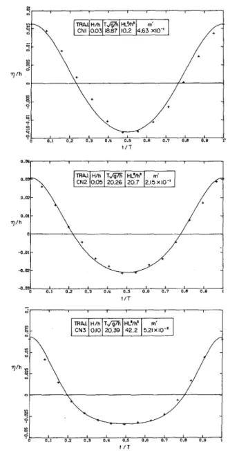
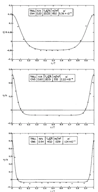
Waves generated using the wave plate trajectories shown in Figure 9 are compared to theoretical wave profiles in Figures 13a and 13b. In these figures the corresponding conditions are shown in each portion of the figures; it is noted, the Ursell Number (HL2/h3) for these experi- ments varies by two orders of magnitude from 10 to 1229. The experi- mental record was obtained from a wave gage located between 5 and 20 depths from the wave plate (x = 1.0 m). In an attempt tq minimize the effects of both the leading and the trailing part of the wave train, the data shown are for the third cycle in the wave train. The wave height which was measured was used to construct the theoretical profile; thus, reducing the effect of friction during propagation and disagreements with the generation theory as embodied in Equation 16. Therefore, only the shape of the wave is being compared in Figures 13a and 13b. It appears that agreement between the experimental and theoretical results is relatively good with discrepancies apparent primarily in the region of the trough, especially for the cases of large Ursell Number.

In Figure 14 experimental and theoretical results are presented which summarize the generation theory for long waves. The ordinate is the ratio of wave height to stroke, H/S, and the abscissa is a non- dimensional wave period, (l/T)(/h/g). Shown in the figure are curves of constant wave height-to-depth, H/h, and of constant nondimensional time, t0/T, which describe the time to the maximum of the trajectory as shown in Figure 8. Thus, for a desired wave height* wave period, and depth, the stroke of the wave machine and the time to the maximum of the trajectory can be obtained. It is noted that the Tine which emanates from the origin describes small amplitude shallow water waves and the curve t0/T = 0.25 is tangent to it. The intersection of curves of constant H/h with the ordinate describe the generation of solitary waves. Experimental data are presented for periodic waves in Figure 14 where the symbols correspond to particular values of wave height-to- depth and relative time to the extreme of the trajectory, t0/T. Thus, the comparison can be made between the data and the curves of constant relative wave height, H/h, and constant relative duration, t0/l.: It is apparent that agreement increases with increasing t0/T and decreasing H/h. Considering the shape of the trajectories this would be expected.

&

A

-^\*

_V

_\

'

\ /

-

I

\, /

-

,

^

\

-

\ /

-

0 0.1 0.2 0.3 O.l) O.S 0.6 0.7 O.B O.S 1 t/T Tj/h , TRW. CN3 H/h 0.10 Vg7h 20.39 HL'/h! 42.2 m' 5.21 XIO"2

-

/ -

/

y

Figure 13a Comparison of the shape of experimental cnoidal waves with theory. (Trajectories CNI, CN2 and CN3)

17"/h 0.05 TRAJ. cm 0.20 H/h Tv57Fi 20.33 HL'/h' 85.0 m' 5.38 x 10"'

-

-

-

-

^/

Figure 13b Comparison of the shape of experimental cnoidal waves with theory. (Trajectories CN4, CN5 and CN6)

\ N\ \ —A

\

'

— \

\ \ ^

_{\ \ V^}

V \ f\

\ \ \V

\ *v\

-

s

1

<

-

_\

\ *\

v \

A* \

-

\-^y

-

\

\ vfc"*

-

\ ""A

-

-

_{\ \ \ ^}

\

CONCLUSIONS

This study has shown the importance of considering the position of the wave plate relative to the position of the generated wave in a long wave generation model. If this is done, quite acceptable profiles for solitary and cnoidal waves- are possible.

ACKNOWLEDGMENTS

This study was supported by NSF Grant Nos. ENV72-03587 and ENV77-20499 and by the New Zealand Ministry of Works and Development. It was carried out while the junior author was a graduate student at the California Institute of Technology as part of his Ph.D. thesis.

REFERENCES

Boussinesq, J. (1872), "Thgorie des Ondes et des Remous qui se Propagent le Long d'un Canal Rectangulaire Horizontal, en Communiquant au Liquide Contenu dans ce Canal de Vitesses Sensiblement Parreilles de la Surface au Fond," Journal de Mathematiques Pures et Appliquges, 2nd Series, Vol. 17, pp. 55-108.

Fenton, J. (1972), "A Ninth-Order Solution for the Solitary Wave," Journal of Fluid Mechanics, Vol. 52, Part 2.

French, J. A. (1969), "Wave Uplift Pressures on Horizontal Platforms," W. M. Keck Laboratory of Hydraulics and Water Resources, Report No. KH-R-19, California Institute of Technology, Pasadena, CA.

Goring, D. G. (1978), "Tsunamis - The Propagation of Long Waves Onto a Shelf," Report No. KH-R-38, W. M. Keck Laboratory of Hydraulics and Water Resources, California Institute of Technology, Pasadena, CA. Hammack, J. L. and Segur, H. (1974), "The KdV Equation and Water Waves. Part 2. Comparison with Experiment," Journal of FluichMechanics,

Vol. 65, pp. 289-314. :

McCowan, J. (1891), "On the Solitary Wave," London, Edinburgh and Dublin Philosophical Magazine, Vol. 32, pp. 45-58.

Segur, H. (1973), "The Korteweg-de Vries Equation and Water Waves. Part 1. Solutions of the Equation," JournaT-of Fluid Mechanics, Vol..59, pp. 721-736.