Unsupervised Data Classification for Convex and Non Convex Classes

Unsupervised Data Classification for Convex and

Non Convex Classes

Fairouz Lekhal

LABO LEPAS, FS, University Mohammed I, MAROC

Mohamed El Hitmy

LABO LEPAS, FS, University Mohammed I, MAROC

Ouafae El Melhaoui

LABO LEPAS, FS, University Mohammed I, MAROC

ABSTRACT

We present in this work, a new unsupervised data classification technique based on a three steps system: Split, Clean and M erge. In this system, the classes are represented by a set of subclasses that we call prototypes. The prototypes are created in an incremental way from the initial data set. No prior knowledge on the classes is required. The data are presented to the system one by one in an arbitrary way. The system built on a neural network strategy ends up by acquiring knowledge on the data and gathers the data into a set of real classes which may have a non convex structure. The method proposed is compared to the fuzzy C-means ‘FCM’ and fuzzy min max clustering ‘FMMC’ methods through a number of simulations. The results obtained by the proposed method are very good.

Keywords

U

1.

INTRODUCTION

Unsupervised data classification is an important technique in the field of data analysis; it has played an important role in many scientific fields. The objective of unsupervised data classification is to regroup the data into classes according to a similarity criterion. The data are not labeled and no prior knowledge on the classes is available [1] [10].

Several methods for unsupervised data classification are already very common and these include [4]: hierarchical, partitioning, connexionist, by tree, by graph … etc. The most common among these are the partitioning methods. The algorithms used in partitioning methods include: C-means [5], Fuzzy C-means [6] [11], Isodata [7], competitive neural network [5]… etc. These algorithms optimize iteratively a classification criterion, in order to partition a set of observations into a set of classes. The drawback with these algorithms is to initially set arbitrarily the number of classes C to a certain value and the value of C is varied until optimality is achieved. Optimality criteria such as Xie and Beni, entropy and partition coefficient are commonly used [8] [11]. Another drawback is the initialization of centers. Starting the algorithm with a different initial value yield to another convergence point different from the first one. Authors have proposed evolutionary algorithms in order to get around these two drawbacks [5] [10]. C-means, fuzzy C-means and competitive neural networks are well suited to convex classes having spherical or elliptical structures; they are not convenient to non convex or complex classes. M any authors have been interested to such a type of problem, regarding the form of the classes, they have proposed a multitude of methods based on existing data classification methods, such as SVM [13], Fuzzy

pattern matching FPM [11], neural networks [12]…etc. The most commonly used algorithm for this problem remains however the one proposed in [3] which is based on a neural network structure and called fuzzy min max clustering FMMC.

In this work, we propose a new method for unsup ervised data classification, which prove to be valid for convex and non convex type of classes. The method is based on three steps: split, clean and merge. The split technique is based on a neural network with evolving architecture; the network contains two layers which will make it possible to divide the data into several prototypes in an incremental way. The prototypes obtained are characterizing elements of the real classes. The clean step discards the noisy prototypes, which are non representative of the real classes. M erge step is an algorithm based on an evolving neural network, constituted of three layers. The merge technique is well adapted for regrouping the similar prototypes into end classes by means of a merge procedure after that the clean operation has been performed.

2.

FUZZY CLASSIFICATION

2.1.

Descriptive elements

Let’s consider a set of M objects {O1, O2,..,Oi, .., OM }, characterized by N parameters regrouped in a line initial vector Vinit = (a1, a2, .., an, .., aN). Let Ri = (ain)1≤n≤N be a line vector of RN _{where the n}th _{component a}

in is the value taken by an for the object Oi. Ri is called the observation associated with Oi. RN is the observation space, or the parameters space. Let EV = {a1, a2, .., an, .., aN} be the set of attributes associated with Vinit.

2.2.

Fuzzy C-means algorithm.

Let’s consider M observations (Ri)1≤i≤M to be associated to C

different classes (CLs)1≤s≤C with respective centers (xs)1≤s≤C .

Fuzzy C-means algorithm FCM associates with each observation Ri its membership degree μis, to the class CLs. μis

[0, 1]. FCM method consists of determining the class centers which minimize the optimization criterion defined by [5] [10]:

 

1 1

s i df M

i C s

is

m R x

J 



 



Under the constraints:





 C

s is

1

1

 for i=1 to M and 0 <





M

i

is

1





 

   



 _

   



 _

 C

k

df k i

df s i is

x R

x R

1

1 1 2

1 1 2



 

 





 



M

i

df is

i M

i

df is

s

R

x

1 1





Despite the simplicity and the popularity of this algorithm, it suffers from the same drawbacks as the C-means does. These are: the number of classes must be known a priori, the initialization problem and the possibility that the convergence point may stack on a local rather than on a global optimum [8] [10] [11].

2.3.

Fuzzy min max clustering

In 1993 Simpson introduces the neural algorithm known as fuzzy min max clustering FMMC [3]; it is a neural network based algorithm with evolving architecture. It is based on unsupervised learning rules which were in itially developed by the same author in 1992 for supervised classification based on a neural fuzzy min max approach [2]. FMMC contains three layers, input, output and hidden layers. The number of neurons in the input layer is equal to the dimension of the data representation space; it is the space RN where N is the size of the attribute vector giving the features of the data. The numbers of neurons in the hidden and output layers increase in time with respect to the creating of prototypes for the hidden layer and creating of classes for the output layer. The synaptic weights associated with the connections between input and hidden layers are formed by two matrices V and W giving the characteristics of the different prototypes in the hidden layer. The synaptic weights associated with the connection between hidden and output layers are formed by a Z matrix characterizing the association of prototypes to the classes. The learning process is made in three steps, expansion overlapping and contraction.

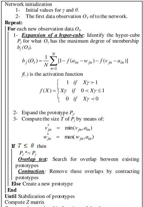
The main objective of this algorithm is to characterize the real classes by a set of fuzzy hyper-cube prototypes, without prior knowledge on the classes. Each prototype Pj is defined by a couple of points (Vj, Wj), where Vj = (vjn)1≤n≤N and Wj = (wjn)1≤n≤N, corresponding respectively to the prototypes influence zone min max. Two parameters need to be fixed before starting the algorithm, the sensitivity γ and the vigilance factor θ of the hyper-cube. FMMC algorithm steps are shown in figure 1:

Network initialization

1- Initial values for γ and θ.

2- The first data observation O1 of to the network.

Repeat:

For each new observation data Oi,

1- Expansion of a hyper-cube: Identify the hyper-cube

Pj for what Oi has the maximum degree of membership bj (Oi).





    

N n

in jn jn in i

j f a w f v a

N O b

1

)] (

) (

1 [ 1 ) (

f(.) is the activation function

    

 

0 0

1 0

1 1

) (

 



  



X if

X if X

X if X

f

2- Expand the prototype Pj.

3- Compute the size T of Pj by means of:

) , max(

) , min(

* *

in jn jn

in jn jn

a w w

a v v

 

If then Pj *= Pj

Overlap test: Search for overlap between existing

prototypes

Contraction: Remove these overlaps by contracting

prototypes

Else Create a new prototype

End

Until Stabilization of prototypes Compute Z matrix

Compute the membership functions of the classes. Fig 1: FMMC algorithm.

The FMMC algorithm suffers however from the quality of the adopted model [12]. The hyper cube mode is a loose approximation of the data distribution. Tuning with γ and θ parameters does not solve this problem. Big value for γ gives rise to an over learning while taking θ as a s mall value creates a lot of prototypes.

3.

PROPOSED METHOD

The proposed method is shown in figure 2:

Fig 2: Proposed method.

The objective is to characterize each class by a set of well representative prototypes in an unsupervised way. Each prototype is represented by a set of data points defining a cloud of loosely a spherical form. The prototype is characterized by the gravity center of all the data points it contains. Three threshold points must be set out initially in order to obtain the prototypes and the classes. These are SSplit, SClean, and SMerge, the three thresholds for the operations Split, Clean and M erge act as decision parameters respectively. A

Merge

Clean

H (H≤S) the most representatives

prototypes Real K

classes Observation

set

data observation Oi is considered to belong to a prototype Pj if the distance between Oi and the gravity center of Pj is lower than SSplit. Setting SSpl it to a correct value is not an easy task. It is an application dependant problem. We have set it here, in this work, to a small value in the hope to divide the data into subclasses (prototypes) of very similar points. This is at the expense of obtaining a lot of prototypes. SClean is a threshold for clean operation. Its task is to remove the bad prototypes. A prototype is considered, in this work to be bad if it contains a reduced number of data. In this case we considered those prototypes with cardinal values less than SClean as candidates to be removed. SMerge is a threshold parameter designated to merge similar prototypes. We considered the distance between two prototypes to be the minimum distance between all the data points in the two prototypes.

d(Pi, Pj)=min({d(x, y), x Є Pi, y Є Pj})

Two prototypes Pi and Pj are merging into one subclass if the distance between Pi and Pj is lower than SMerge. We have set SMerge to a small value in order to only merge those prototypes which are very similar.

3.1.

Split algorithm

The Split phase is accomplished through a neural network with evolving architecture, figure 3. The network contains two layers. An input layer with N neurons representing the realization of the object Oi, Ri=(ai1,…, ain,…, aiN) where ain are the attribute elements. An output layer having a number of neurons defining the exiting prototypes in a giving instant of time. Each prototype Pj is characterized by a neuron in the output layer. The size of this layer is not fixed initially, it increases with time as long as new p rototypes are created when new observation data points is applied to the network. The output layer is fully connected to the input layer. The synaptic weight associated with the connections W corresponds to the gravity centers of the existing S prototypes. W

Fig 3: S plit neural network architecture.

Mode of operation of the Split process.

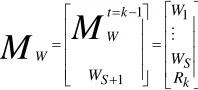
Initially at t=0, observation O1 is applied to the network. Output layer contains one neuron and the matrix of synaptic weights Mw is:

MW = W1= [w11 w12…. w1n ….. w1N] = [R1] = [a11 a12 …a1n… a1N]

R1 is the realization of the data point O1, figure 4. P1 is formed by O1.

w11 w12

w1n

w1N

Fig 4: Configuration of the network associated with S plit phase at t=0

At iterative t=1, the distance between R2 and W1 is computed, R2 is the realization of O2, O2 is the second data point.

If d(R2,W1) ≤SSplit , then O2 is attributed to P1 and the synaptic weight vector W1 becomes :

2 ) (

2 1 1

1 1

R R P card

R

W R P

i

i  







If d(R2,W1) >SSplit, then O2 is not in P1, A new prototype P2 and a new neuron are created (figure 5). The new prototype is characterized by the attribute vector associated with O2 and the synaptic weights matrix becomes

Where: the weight matrix at t=0. W

Fig 5: Creation of a new prototype

Proceeding with the algorithm, we consider that at iteration t=k-1, we obtain S prototypes associated to S neurons in the network output layer. We pass on to iteration t=k, object Ok is applied to the network’s input layer through its realization Rk, the distance between Rk and the various Wj are computed, for j=1 to S, let Wr be the closest to Rk,

d(R_k,W_r)minS_j1(d(R_k,W_j))

If d(Rk,Wr) ≤ SSplit then Ok is attributed to Pr and the synaptic weight vector associated to neuron Pr becomes:

)

(

i r

P

card

R

W







The synaptic weights associated with the other neurons j≠r, remain unaffected. .

If d(Rk,Wr) > SSplit, then Ok is far away from all the existing prototype at t=k-1. In this case a new prototype PS+1 and a new neuron are created in the network’s output layer. PS+1 is characterized by Rk and the weight matrix is:

3.2.

The clean operation

Finishing off the Split phase, many prototypes sometimes by hundreds are produced. Among the obtained prototypes in the split phase, many of them are non representatives of the real classes and must simply be removed without causing any harm to the initially pointed out objective. Indeed the presence

          

 

   

  



2 1

2 0

R W W

M

M

t W W

   

 

   

 

    

 

   

  

  

k S S

k t W W

R W W

W

M

M

1

1 1

a1 a2

an

aN

P1 P2

Pj

PS

a21 a22

a2n

a2N

P1 P2

a11 a12

a1n

a1N

P1

P2

Pj

PH

P1

P2

Pj

PH of these non representative prototypes does not improve the

discrimination between the classes and the information they add for representing the classes is negligible if compared to the noise they generate.

In order to avoid this problem, we opted for a clean operation where we delete the non representative prototypes. In this work, the cardinality of the prototype is used as a criterion for removing or keeping the prototype. If the cardinal of a prototype is less than SClean then the prototype is considered be non representative and is removed. SClean is a threshold parameter which is set out initially and is taken as a small value after an error and trial procedure.

3.3.

The Merge algorithm

The split procedure described previously obtains a high number of prototypes. The main reason for this is that the split algorithm divides the observations in an arbitrary way. The solution is to merge similar prototypes into one. The similarity between prototypes is defined by a similarity criterion based on a distance measure [11]. M erge algorithm is a neural network with evolving architecture figure 6. The network is formed by three layers.

U V

Fig 6: Merge neural network architecture.

The input layer is made of H neurons, where H is the number of prototypes found after the clean operation. The hidden layer is also formed by H neurons corresponding to the H prototypes, the input and hidden layers are fully connected by means of a binary matrix U=(ui j )(1≤i≤H,1≤j≤H), where uij define the connexity between the prototypes Pi and Pj. The distance between two prototypes Pi and Pj is defined by [4]:

d(Pi, Pj)=min({d(x, y), x Є Pi, y Є Pj})

If J(Pi, Pj)≤ SMerge then Pi is considered to be similar to Pj and uij =1.

If J(Pi, Pj)>SMerge the two prototypes are considered to be not similar and uij =0.

The output layer contains a number of neurons defining the real existing classes. Each class Ck is characterized by a neuron on the output layer. The number of neurons on the output is not fixed initially, the algorithm starts with one neuron, and the number of neurons increases with time in correspondence with the creation of classes where similar prototypes are regrouped. Hidden and output layers are fully connected by means of a binary matrix V=(vjk)(1≤j≤H,1≤k≤K),. The prototype Pj is considered to be a member of the class Ck if vjk=1, if not, vjk =0. vjk=1 in two cases, the first case is when the algorithm chooses to open a new class Ck because Pj is not connex to any of the previous k-1 classes, the second case is when Ck is already existing and Pj is connex to one of the elements of Ck.

Mode of operation of the Merge process

At iteration t=0, the architecture of the merge network is that of figure 7, one neuron at the output layer corresponding to a real class C1. C1 contains P1 and all the prototypes which are

directly or indirectly connex to P1. Two prototypes Pa and Pb are indirectly connex if there exists a chain of prototypes related by a connexity relationship where the two prototypes Pa and Pb are present. For example, consider the chain:

P1 P2 P3 P4

P1 is directly connex to P2 but it is indirectly connex to P3 and P4.

U V

Fig 7: Configuration of the network associated with Merge phase at t=0

At iteration t=k-1, the output layer contains k-1 neurons corresponding to k-1 real classes.

At iteration t=k, the algorithm looks for the first prototype not yet classified, the search is looked at in an increasing way from P1, upwards until Pj where Pj does not belong to neither of the k-1 already set classes. This means that (vjc)(1≤c≤k-1) are all equal to zero. A kth neuron is then added to the output layer characterizing the class Ck and containing Pj and those prototypes which are not yet classified and which are directly or indirectly connex with Pj. This process is carried out until all the prototypes are attributed to their specific classes.

4.

EXPERIMENTAL RESULTS

Two experiments are carried out in this section, one considers classes of convex type and the classes are non convex for the second one. The data for both experiments are represented in a two dimensional space.

4.1

First experiment: Classes of convex

form.

In this experiment, two types of simulation are carried out. For both simulations the classes have convex form, we have three classes in each case, and the data have been generated by a Gaussian distribution routine through M atlab. The difference between the two simulations can be seen in the number of data, the level of overlapping between the classes and the noisy data introduced in the second simulation. For both simulations we set SSplit=0.8, SClean=10 and SMerge=0.2

4.1.1

Simulation 1

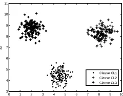
The data to be classified for this simulation are shown in figure 8. The overlapping between the classes in this case is

null, the noisy data are not there, each class contains 150 data.

Fig 8: Repartition of the classes in the observation space.

The Split phase runes quickly and obtains 14 prototypes. In the clean process three prototypes are removed. The 11

0 1 2 3 4 5 6 7 8 9 10 3

4 5 6 7 8 9 10 11

a1

a2

Classe CL1 Classe CL2 Classe CL3 P1

P2

Pj

PH

C1

Ck

CK

P1 P2

Pj

PH

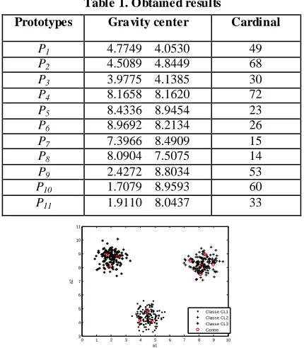
remaining and most representative prototypes are gathered in the set ES = {P1, P2, P3, P4, P5, P6, P7, P8, P9, P10, P11}. Table 1 and figure 9 show the results obtained.

Table 1. Obtained results

Prototypes Gravity center Cardinal

P1 4.7749 4.0530 49

P2 4.5089 4.8449 68

P3 3.9775 4.1385 30

P4 8.1658 8.1620 72

P5 8.4336 8.9454 23

P6 8.9692 8.2134 26

P7 7.3966 8.4909 15

P8 8.0904 7.5075 14

P9 2.4272 8.8034 53

P10 1.7079 8.9593 60

P11 1.9110 8.0437 33

0 1 2 3 4 5 6 7 8 9 10 3 4 5 6 7 8 9 10 11 a1 a2 Classe CL1 Classe CL2 Classe CL3 Centre

Fig 9: Prototypes with corresponding centers obtained by the proposed method.

The set Es is applied to the M erge algorithm. The synaptic weights between the hidden and output layers obtained at convergence are            1 1 1 0 0 0 0 0 0 0 0 0 0 0 1 1 1 1 1 0 0 0 0 0 0 0 0 0 0 0 1 1 1 V

Convergence is achieved when the output layer contains three neurons. Each neuron represents a real class which is formed by several prototypes. The number of classes obtained is then 3 which coincides with the true one. The repartition of prototypes in the classes is:

 CL1= {P1, P2, P3}  CL2= {P4, P5, P6, P7, P8}  CL3= {P9, P10, P11}

4.1.2

Simulation 2

The second simulation is illustrated by figure 10. There is some overlapping between the classes and many noisy data in each class are there. Each class are there contains 250 observations.

-2 0 2 4 6 8 10 12 0 2 4 6 8 10 12 a1 a2 CL1 CL2 CL3

Fig 10: Repartition of the classes in the observation space.

The split process runs quickly and obtains 70 prototypes. The clean operation removes 38 prototypes and 32 prototypes remain as the most representatives of the real classes. The final stage is the merge process which obtains at convergence a synaptic weight matrix between hidden and output layers given by:

           0 0 0 0 0 0 0 0 1 1 1 1 1 1 1 1 1 1 1 0 0 0 0 0 0 0 0 0 0 0 0 0 1 1 1 1 1 1 1 1 0 0 0 0 0 0 0 0 0 0 0 1 1 0 0 0 0 0 0 0 0 0 0 0 0 0 0 0 0 0 0 0 0 0 0 0 0 0 0 0 0 0 0 0 0 1 1 1 1 1 1 1 1 1 1 1 V

The algorithm obtains 3 neurons for the output layer; we then obtain three real classes which coincide with the true number of classes. The repartition of prototypes between the classes is:

CL1= {P1, P2, P3, P4, P5, P6, P7, P8, P9,P 10, P11} CL2= {P12, P13, P25, P26, P27, P28, P29, P30, P31, P32} CL3= {P14, P15, P16, P17, P18, P19, P20, P21, P22, P23, P24} Figure 11 shows graphically the obtained results for data classification.

-2 0 2 4 6 8 10 12 0 2 4 6 8 10 12 a1 a2 CL1 CL2 CL3 Centre

Fig 11: Prototypes and their corresponding centers obtained by the proposed method.

4.1.2.1 Comparison with the FCM

The aim is to compare the proposed method with the FCM. The comparison is conducted through simulation 2 case study. Unsupervised FCM classification does not know what is the number of classes initially. Several criteria have been proposed in the literature for optimally selecting this number. We have chosen the Xie and Beni criterion which make use of compacity and separability notions [10]. The FCM algorithm is run for several values of C (number of classes) and the Xie and Beni criterion value FXB is computed for each value chosen for C. figure 12 shows the evolution of FXB with respect to the number of classes.

2 3 4 5 6 7 8 9 200 300 400 500 600 700 800 900

Le nombre C

F

x

b

Fig 12: Evolution of FXB with respect to the number of

classes.

knowing the number of classes has converged to the optimal solution.

We take C=3 for FCM and carry out a comparison between the two methods. The results obtained are summarized in table 2.

Table 2: Classification results number of misclassified observations

Classifcation rate

FCM (C=3) 24 96.8%

Proposed method 18 97.6%

A higher classification rate is obtained by the proposed method. 18 observations were misclassified by the proposed method from among the initial 750 ones, and a classification rate of 97.6%, the CMF has obtained 24 observations misclassified and a classification rate of 96.8%.

4.1.2.2 Comparison with fuzzy Min Max clustering

FMMC

We have compared the proposed method with FMMC through simulation 2. Figure 13 shows the classification results obtained for FMMC method. Table 3 shows the performances of the two methods.

-2 0 2 4 6 8 10 12 0

2 4 6 8 10 12

a1

a2

Fig 13: Prototypes obtained by the FMMC method.

The number of classes obtained by FMMC does not coincide with the true one; this is due to the high overlapping between the classes where prototypes are created in the overlapping zone which mix all the classes to one. For the proposed method the clean operation has acted in such a way that the classes have remained separated. We also noticed that the running time of FMMC method is largely greater than that for the proposed method.

4.1.2.3 Case with noisy data

We are interested to study the behaviors of the proposed method when there one a lot of noisy data embedded in the set of initial data to be classified, and when the degree of overlapping between the classes is high. We have used the data of simulation 2 to which we have added 150 noisy observations. Figure 14 and table 4 show the results obtained by the proposed and FCM methods.

-4 -2 0 2 4 6 8 10 12 0

2 4 6 8 10 12

a1

a2

CL1 CL2 CL3 Noisy data Center

(a)

-4 -2 0 2 4 6 8 10 12 0

2 4 6 8 10 12

a1

a2

CL1 CL2 CL3 Noisy data Center

(b)

Fig 14: (a) Prototypes obtained by the proposed method. (b) Prototypes obtained by FCM.

Table 4: Results of data classification number of

misclassified observations

Classifcation rate

FCM (C=3) 30 96%

Proposed method 18 97.6%

The classification for FCM has slightly decreased due to the noisy data effect, while it remains the same as in 4.1.2.1 for the proposed method.

4.2

Second experiment: Classes of non

convex or complex form.

We have envisaged for this experimentation two simulations, each of them considers two classes of non convex form. The form in simulation 3 is rectangular while it is circular for simulation 4. The observation space for the two simulations is of dimension 2. The data have been synthesized by authors and this has made use of the rand routine in M atlab. For both simulations we set SSplit=0.6, SClean=10 and SMerge=0.2

4.2.1

Simulation 3

Simulation 3 uses 1200 observations distributed into two classes of rectangular non convex form as shown in figure 15. Each class contains 600 observations.

0 1 2 3 4 5 6

-1 -0.5 0 0.5 1 1.5 2 2.5 3 3.5 4 4.5

a1

a2

CL1 CL2

Fig 15: Distribution of data in the observation space .

Split algorithm runs quickly and obtains 22 prototypes. The clean operation removes one of them. The 21 remaining

Table 3. Comparison between the two methods.

Number of classes

Learning time

Number of prototypes

FMMC 1 22,6 s 278

Proposed method

prototypes are applied to the merge algorithm and the V matrix obtained is:

   

  

0 0 1 1 1 1 1 1 1 1 1 1 1 0 0 0 0 0 0 0 0

1 1 0 0 0 0 0 0 0 0 0 0 0 1 1 1 1 1 1 1 1

V

The merge algorithm obtains two neurons in it s output layer and the repartition of the prototypes obtained for each neuron is:

CL1= {P1, P2, P3, P4, P5, P6, P7, P8, P20, P21}

CL2= {P9, P10, P11, P12, P13, P14, P15, P16, P17, P18 , P19} Figure 16 shows the obtained results.

0 1 2 3 4 5 6

-1 -0.5 0 0.5 1 1.5 2 2.5 3 3.5 4 4.5

a1

a2

CL1 CL2 Centre

Fig 16: Prototypes and their corresponding centers obtained by the proposed method.

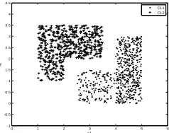
The results obtained by the proposed method are compared to those obtained by FCM and FMMC, figure 17 and table 6.

0 1 2 3 4 5 6

-1 -0.5 0 0.5 1 1.5 2 2.5 3 3.5 4 4.5

a1

a2

CL1 CL2 Centre par CMF

(a)

0 1 2 3 4 5 6 -1

-0.5 0 0.5 1 1.5 2 2.5 3 3.5 4

a1

a2

(b)

Fig 17: (a) Prototypes obtained by the FCM. (b) Prototypes obtained by FMMC.

Table 6 : Classification results

Numbe r of classes

Learning time (s)

Numbe r of prototypes

Classification rate

FCM (C=2) 2 3,34 2 98.5%

FMMC 2 23,6 229 100%

Proposed method

2 1,07 21 100%

Both FMMC and the proposed method have obtained better results than FCM, but the running time for FCM and FMMC are much bigger than that required by the proposed method.

4.2.2

Simulation 4

In this simulation, we have used 1050 observations distributed into 2 classes of circular non convex form (figure 18). The first class contains 100 observations and the second one contains 950 remaining observations.

1 2 3 4 5 6 7 8 1

2 3 4 5 6 7 8

a1

a2

CL1 CL2

Fig 18: Distribution of data in the observation space.

Split algorithm runs quickly and obtains 17 prototypes. The clean operation does not remove any of the prototypes and the V matrix obtained is:

   

  

1 1 0 0 0 0 0 0 0 0 0 0 0 0 0 0 0

0 0 1 1 1 1 1 1 1 1 1 1 1 1 1 1 1

V

The merge algorithm obtains two neurons in its output layer and the repartition of the prototypes obtained for each neuron is:

CL1= {P1, P2, P3, P4, P5, P6, P7, P8, P9, P10, P11, P12, P13, P14, P15}

CL2= {P16, P17}

Figure 19 shows the obtained results.

1 2 3 4 5 6 7 8

1 2 3 4 5 6 7 8

a1

a2

CL1 CL2 Centre

Fig 19: Prototypes and their corresponding centers obtained by the proposed method.

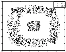
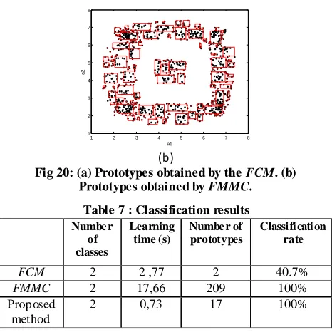
The results obtained by the proposed method are compared to those obtained by FCM and FMMC, figure 20 and table 7.

1 2 3 4 5 6 7 8

1 2 3 4 5 6 7 8

a1

a2

CL1 CL2 Centre par CMF

1 2 3 4 5 6 7 8 1

2 3 4 5 6 7 8

a1

a2

(b)

Fig 20: (a) Prototypes obtained by the FCM. (b) Prototypes obtained by FMMC.

Table 7 : Classification results

Numbe r of classes

Learning time (s)

Numbe r of prototypes

Classification rate

FCM 2 2 ,77 2 40.7%

FMMC 2 17,66 209 100%

Proposed method

2 0,73 17 100%

FCM has failed in this case because the center of classes obtained by FCM is not good. FMMC and proposed method have both converged to the true solution but the running time of the FMMC is largely high than that required for the proposed method.

5.

CONCLUSION

In this work, we have proposed a new method of unsupervised data classification based on a cascade sy stem containing three blocks: split, clean and merge processes. The split process divides the initial set of data into several subclasses; it is based on a neural network containing two layers which builds the subclasses in a progressive way. The clean operation removes the non representative subclasses which contain noisy data; the cardinal value of these subclasses is small. M erge process regroups similar subclasses into a real class according to a chosen similarity criterion. The proposed method have been validated through many examples studied by simulations, the form of the classes chosen for these simulations is convex for some of them and non convex for the others. The results obtained are good; the method has always converged to the optimal solution in a reduced running time. The simulation results have shown that although the degree of overlapping between the classes is high and although the noisy data are present in the initial set of data the method proposed still converge to the expected result. The method does not infer any initial knowledge on the classes especially the number of classes is not initially set by the method. This number is obtained after that the method converges. The simulation results have also shown a net improvement obtained by the proposed method when it is compared to the FCM and FMMC methods of classification.

6.

REFERENCES

[1] P. Jiang, F. Ren and N. Zheng. 2009. A new approach to data clustering using a computational visual attention model. International Journal of Innovative Computing, Information and Control Volume 5, Number 12(A). (December 2009)

[2] P.K. Simpson. 1992. Fuzzy min-max neural networks. Part 1: classification. IEEE Transactions on Neural Networks, vol. 3, pp: 776-786.

[3] P.K. Simpson. 1993. Fuzzy min-max neural networks. Part 2: clustering. IEEE Transactions on Fuzzy Systems, vol. 1(1), pp: 32-45.

[4] M . Boubou. 2007. Contribution aux méthodes de classification non supervisée via des approches prétopologiques et d’agrégation d’opinions. Thése de Doctorat, Université Claude Bernard – Lyon I. [5] H. Ouariachi. 2001. Classification non supervisée de

données par réseaux de neurones et une approche évolutionniste: application à la classification d’images. Thèse de doctorat, Université M ohamed 1, M aroc [6] M . Nasri, M. El Hitmy, H. Ouariachi and M .

Barboucha. 2003. Optimization of a fuzzy classification by evolutionary strategies’’. In proceedings of SPIE Conf., 6th international Conference on Quality Control by Artificial Vision, Vol. 5132, pp. 220-230, USA, 2003. Repulished as an SM E Technical paper by the Society of manufacturing engineers (SM E), Paper number M V03-233, ID TP03PUB135, Dearborn, M ichigan, USA, pp. 1-11, (24 June 2003).

[7] L. Khodja. 1998. Contribution à la classification floue non supervisée. Thése de doctorat, université de savoie.

[8] K. R. Zalik and B. Zalik. 2010. Validity index for clusters of different sizes and densities. Pattern Recognition Letters, 221-234, (18 September 2010). [9] C. Duo, L. Xue and C. Du-Wu. 2007. An Adaptive

Cluster Validity Index For The Fuzzy C-means. IJCSNS International Journal of Computer Science and Network Security, VOL.7 No.2, ( February 2007). [10] M . Nasri. 2004. Contribution à la classification des

données par approches evolutionnistes : simulation et application aux images de textures. Thèse de Doctorat, Université M ohammed premier, Faculté des sciences Oujda, M aroc.

[11] M . S. Bouguelid. 2007. Contribution à l'application de la reconnaissance des formes et la théorie des possibilités au diagnostic adaptatif et prédictif des systèmes dynamiques. Thése de doctorat, Université de Reins Champagne- Ardenne.

[12] H. A. Boubacar. 2006. Classification dynamique de données non-stationnaires apprentissage et suivi de classes evolutives. Thése de doctorat, université des sciences et technologies de lille.