ABSTRACT
The goal of this paper is to propose a method for carrier frequency offset estimation in a scenario where multiple users upload to a central coordinator simultaneously. OFDM based systems are highly prone carrier frequency offsets. The CFO estimation method proposed here is performed in time domain thereby facilitating a reduction in complexity at the central coordinator. The estimator makes use of the orthogonal training sequences that were transmitted by the different users. It is shown that the resulting CFO estimator is optimal not only in the sense that it minimizes the estimation error variance due to inter carrier interference.
General Terms
Multiple input multiple output, OFDM orthogonal frequency division multiplexing.
Keywords
Wireless local area networks, cyclic prefix, carrier frequency offsets, Central Coordinator.
1. INTRODUCTION
Orthogonal frequency division multiplexing has found applications in various digital communication systems, such as digital audio/ video broadcasting and wireless local area networks (WLAN). Compares with single carrier systems, OFDM is more sensitive to carrier frequency offsets, so accurate estimation and compensation of CFO is very important. Most CFO estimators rely on periodically transmitted pilots “Ref [1, 2]’’ One class of blind CFO estimators take advantage of the null sub carriers existing in many OFDM systems “Ref [3, 4, 5,6]’’. These estimators are robust against channel multipath, but have relatively high computational costs. On the other hand, blind estimators utilizing the cyclic prefix or cyclostationarity of OFDM transmission “Ref [7,8,9,10]’’ have lower complexity but their performance degrades as frequency selectivity becomes more pronounced. The CP based scheme proposed in “Ref [2]’’ is robust against channel multipath, but requires that the cyclic prefix is strictly longer than the channel delay spread and that the exact channel order is known. Here a CFO estimation method is proposed that makes use of the orthogonality among the training sequences transmitted by each of the stations. The degradation in orthogonality gives the measure of the carrier frequency offset.
2.
SYSTEM
MODEL
The multiple CFO estimation is performed using the preamble sequence that contains frequency samples for every station
such that preamble of sequence of a station is orthogonal to all other stations. Assume that K different CFOs are estimated based on the observation of a single received signal. This represents a multi-user MIMO system where the CFOs between each transmitter-receiver pair.
Fig1: Multiple users uploading simultaneously to a single multi-antenna receiver. The users are located at different
distances from the receiver and experience various bounded time delays
T
1toT
MLet us consider a network where the central coordinator (Access Point in WLANS) polls to multiple stations thereby facilitating simultaneous transmission of the polled stations. Once the stations are polled, depending on the time frame, each station has to start transmission with the training sequences all of which are added at the coordinator on reception. The channel that constitutes of a phenomenal Raleigh fading distribution as well as an Additive White Gaussian component corrupts these training sequences prior to reception. The Central Coordinator (CC) has to estimate the respective carrier frequency offsets that it experiences with relative to each of the polled stations. To achieve this, the training sequences transmitted by each of the stations.
Must be interleaved in frequency domain so as to facilitate orthogonality. The CC makes use of this orthogonality for synchronization as well as channel estimation. As a result of the carrier frequency difference among the stations, the individual training sequences lose orthogonality upon down conversion at the CC. Here a method has been proposed,
K.V. Narayanaswamy,
PhD.Member, IEEE
Professor, Head Division of TCLL M.S.R.S.A.S, Bangalore, INDIA
Carrier Frequency Offset Estimation in
Multiuser Simultaneous Channel Access for
where the CC estimates the various CFOs by applying some signal processing techniques on the received signal. The received signal would be the added version of all the training sequences transmitted by different stations. The training sequences used for the estimation consists of 10 identical short symbols that are transmitted back to back. And each symbol is composed of 16 samples. Hence the short training sequence would be periodic every 16 samples. For M stations communicating to the CC, M frequency interleaved short training sequences are required. Let each symbol of the interleaved STSs in time domain be denoted as [s1 s2 s3….. sM].
[image:2.595.53.292.418.518.2]Hence the conventional interleaved structure for the M station system will look like.
Fig 2: conventional STS preamble structure for M station system.
But in the proposed method, a small change has to be made in the above structure in order to estimate each of the CFOs i.e. the symbols must not only be interleaved in sub-carriers but also should be sign inverted. The sign inversion shouldn’t apply to all the symbols in a particular sequence, but only for selected symbols. The following sequence structure includes the symbols where the sign must be inverted.
Fig 3: modified STS preamble.
In the above fig3, the symbols underlined in red indicate those symbols whose sign has to be inverted. The estimator at the CC is designed in the next section.
3.
CARRIER
FREQUENCY
ESTIMATION
Let
x
x
1x
2...
x
M
T be the transmitted short training sequence vectors wherex
m being the STS vectorfrom the mth station, which is of dimension
(
N
1
)
. And N is the total number of samples in the entire STS frame. By convention, N = 160.Let
f
m be the carrier frequency offset experienced at thecentral coordinator with respect to the mth station and
f
mbe its local oscillator frequency of the mth station. The compositebase band signal is unconverted to the RF Passband, which can be described as
m sf
nT j m
m
n
x
n
e
u
(
)
(
)
2 ……. (1)Where Ts is the sampling time. Transmission happens at the same time from all the stations. Hence at the central coordinator, the summed Passband signals will be down converted to the baseband form as shown below.
c sf nT j M
m m
m
n
u
n
e
v
21
)
(
)
(
,Where fc is the oscillator frequency of CC.
If
m represents the relative delay in reception of each of the sequences incurred at the CC due to the physical separation of the stations, to getc sf nT j M
m
m m
m
n
u
n
e
v
21
)
(
)
(
Expanding the above equation using (1),
c s m
s
m j nTf
M
m
f T n j m m
m
n
x
n
e
e
v
21
) ( 2
)
(
)
(
Mm
f f n T j m m
m
m m m s
e
n
x
n
v
1
) (
2
)
(
)
(
The exponential term in the above equation can be used to define C as a CFO matrix of dimension
(
N
N
)
, explained as [image:2.595.329.547.619.741.2])
...
...
(
j2Ts(fm mfm) j2Ts(2fm mfm) j2Ts(Nfm mfm)m
diag
e
e
e
C
…….. (2)
Given correct symbol synchronization, and including the effects of the channel together associated with the imperfect oscillators in the upconversion and downconversion, the received signal vector at the CC in the presence of AWGN can be represented as
η
x
C
y
M
m
m m
1 ^
…… (3)
Where ^
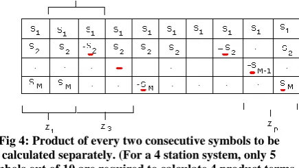
m
x
represents the channel affected STS vector. Defining D as the sample delay between the identical OFDM short training symbols of the received signal. If L is the number of samples in a symbol, consecutive received symbols are multiplied separately so as to design the estimator. The number of products to be taken depends on the number of stations in the system. For M stations, M products are required, hence P = M as shown below.Fig 4: Product of every two consecutive symbols to be calculated separately. (For a 4 station system, only 5 symbols out of 10 are required to calculate 4 product terms
The intermediate value z is developed for the estimator as
L np
y
n
y
n
D
z
1 *)
(
)
(
Where p = 1 to P From (3) get
L n M m m m m M m m m mp C nnx n C n Dn D x n D
z 1 * 1 ^ 1 ^ ) ( ) , ( ) ( ) , (
Considering all the cross products to be negligible due to the orthogonality among the training sequences,
L n M m f DT j m m m m p m se
D
n
x
n
x
z
1 1 2 * ^ ^)
(
)
(
On interchanging the summations, get
M m L n f DT j m m m m p m se
D
n
x
n
x
z
1 1 2 * ^ ^)
(
)
(
Over L samples, ^
m
x
can be represented as m^
s
which is a1
L
vector (see Fig 3).
M m L n f DT j m m m m p m se
D
n
s
n
s
z
1 1 2 * ^ ^)
(
)
(
m ^s
Can be broken down asH
ms
m , where Hmis defined asthe channel circulant matrix of dimension
L
L
given by
1 1 1 2 1 2 2 3 10
...
0
0
0
.
0
...
0
.
0
...
0
....
0
...
0
k k k k k mH
Where
1,
2,...
k
are the time domain channel coefficients
M m f DT j m m m H m m m L np n n D e s m
z 1 2 1 ) ( )
( H s
s H
m
s
is periodic over every L samples. Since D will be either equal to L, or an integer multiple of it, regardless of the delays, due to the periodicity in the short training symbols to get
M m f DT j m m H m mp
W
m
p
Q
m
p
e
s mz
1 2)
,
(
)
,
(
H
s
s
H
Where W (m,p) and Q (m,p) are the sign values of the transmitted short training symbols as indicated in Fig (3).
Rearranging the above equation to get.
M m f DT j m m H m H mp W m p Qm p e s m
z 1 2 ) , ( ) ,
( H s
H s
M m f DT j m m H m H mp
W
m
p
Q
m
p
e
s mz
1 2)
,
(
)
,
(
s
H
H
s
The square of the channel circulant matrix will give another circulant matrix with the diagonal elements taking the highest value. Hence to get
M m f DT j m c m H mp W m p Q m p e s m
z 1 2 ) , ( ) , ( s H s
M m f DT j m c m H mp W m p Q m p e s m
z 1 2 ) , ( ) , ( s H s
M m f DT j m N n m c mp H nn s n W m pQ m pe s m z 1 2 1 2 ) , ( ) , ( ) ( ) , (
M m f DT j m m c m p m se
p
m
Q
p
m
W
n
n
H
z
1 2 2)
,
(
)
,
(
)
,
(
s
M m f DT j m m c m mp H nn W m pQm pe s m
z 1 2 2 2 ) , ( ) , ( ) , ( s s
M m f DT j mp A m W m pQ m pe s m
z 1 2 2 ) , ( ) , ( )
( s
Where A is the scaling factor matrix that resulted due to the channel and Q and W are sign matrices of dimensions
)
(
M
M
each that varies on the sign of the symbols used in the product (shown in Fig 3).
Expanding the previous equation,
M m m s mp
A
m
W
m
p
Q
m
p
j
DT
f
z
1 2)
2
1
(
)
,
(
)
,
(
)
(
s
m s M m m M m m p f DT j p m Q p m W m A p m Q p m W m A z
2 ) , ( ) , ( ) ( ) , ( ) , ( ) ( 1 2 1 2 s s…… (4)
STS symbol samples are the same,
2 2 2
2 2
1
s
...
s
s
s
M
Hence equation (4) can be written as
Mm m
M
m s p
f
p
m
Q
p
m
W
m
A
DT
j
p
m
Q
p
m
W
m
A
z
1
1 2 2
)
,
(
)
,
(
)
(
2
)
,
(
)
,
(
)
(
s
s
--- (5)
The imaginary part of z contains the frequency-offset vector together with the scaling vector Am. However Am can be estimated from the real part of z.
Am contains M number of coefficients. Only on estimation of all the M coefficients will be able to estimate the individual carrier frequency offsets.
From (5) have
2 1
) ( )
, ( ) , ( ) (
s
p M
m
z real p
m Q p m W m
A
2
1 2
) ( )
, ( ) , ( ) (
s
s p m
M
m DT
z imag f p m Q p m W m A
--- (6)
Similarly, performing the same operations on the remaining consecutive symbols, equations (6) will only vary in the sign inversion matrix (due to the sign inversion done on selected symbols at the individual stations as shown in Fig 2), which is known.
And thereby combining all the real terms, one can achieve a number of equations for the same number of unknowns, which in this case is the scaling factor matrix. Once the scaling factor matrix has been estimated, it can be applied on the imaginary parts of the products thereby yielding the carrier frequency offsets. The entire matrix equation can be written as
1)
(
Z
WQ
A
real
ΔF
imag
(
Z
)
AWQ
1Where A and Z are
1
M
(or1
P
) matrices whereas Q, W andΔF
are matrices of dimensionsM
M
(orM
P
).Note that since the number of equation should be equal to the number of unknowns, P = M.
The diagonal elements of
ΔF
will give the respective carrier frequency offsets for m stations.Since the central coordinator is assumed to have the number of antennas equal to the number of stations, carrier frequency offsets can be determined based on the signals received at each antenna, thereby facilitating to take the best result among them.
4.
SIMULATION
RESULTS
Simulation for a scenario with 2 stations communicating with central coordinator has been performed. The individual estimated at the stations. The averaged estimation error of both offsets was plotted against a range of SNR’s. The communication channel CFOs warmed here consists of a dispersive channel together with the additive nature of a Gaussian channel whose SNR is varied throughout the simulation. The number of channels taken into consideration is equal to the square of the number of stations.
CFO
actual
CFO
estimated
CFO
actual
Error
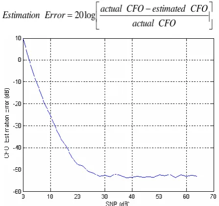
[image:4.595.325.549.83.293.2]Estimation
20
log
Fig 5: SNR vs. CFO estimation Error for a 2-station system with CFOs 50.5 kHz and 16 kHz.
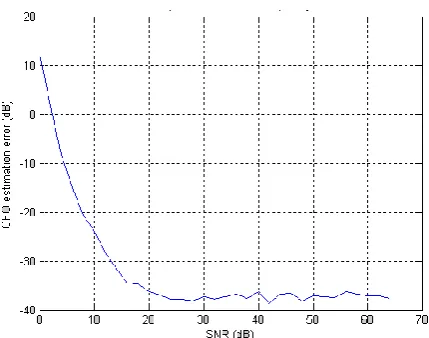
[image:4.595.319.548.472.652.2]As discussed about a delay
being incurred at the central coordinator in the reception of the sequences transmitted by each stations due to their physical separation. The method proposed here has been found to produce fair results even in the presence of such delays. As per the mathematics provided in the previous sections, the cancelled as a result of conjugate multiplication. In a Wi-Fi environment, the range of the access point is the maximum relative delay that would occur among the stations. Ideally the access point range is = 100m ~ samples. The following results exhibit the performance of the algorithm under relative delays of 1, 4 and 7 samples.Fig 6: CFO estimation error vs. SNR for a 2 station system for relative delay = 1 sample, CFOs being
Fig 7: CFO estimation error vs. SNR for a 2 station system for relative delay = 4 sample, CFOs being
30.5 kHz and 70 kHz respectively.
5.
CONCLUSIONS
The precise operating SNR for wireless LAN devices comes in the range 20 to 40 dB over which the CFO estimator presented here performs similar to the estimator used for SISO channels (IEEE 802.11a). The algorithm presented here reduces the effect of Inter-carrier-interference that results due to multiple carrier frequency offset each station experiences with respect to the access point. The CFO estimation error variance is also found to be minimal over a wide combination of frequency offsets.
6.
REFERENCES
[1] P.H Moose, “A technique for orthogonal frequency division multiplexing frequency offset correction”, IEEE trans. Commun, Oct 1994
[2] T.M. Schmidl and D.C. Cox., “Robust frequency and timing synchronization for OFDM”, IEEE trans commun Dec 1997
[3] N. Lashkarian and S. Kiaei, “Class of cyclic based estimators for frequency offset estimation of OFDM systems. IEEE trans. Commun, Dec 2003
[4] X.Ma, C. Tepedelenlioglu, G.B. Giannakis and S. Barabarosa, “Non data aided carrier offset estimators for OFDM with null subcarriers”, IEEE J. Select areas Commun, Dec 2001
[5] G.J Foschini and M. J. Gans, “On limits of wireless commiunications in a fading environment when using multiple antennas”, Wireless personal communications, Mar 1998
[6] J van de Beek, P.O Borjesson, at al, “A time and frequency synchronization scheme for multi user OFDM”, IEEE J. select areas commun Nov 1999
[7] M H Hsieh and CH Wei, “A low complexity frame synchronization and frequency offset estimation scheme for OFDM systems over fading channels”, IEEE Trans. Veh .Tec Sept 1999
[8] X.Ma, G.B. Giannakis, “ Non data aided frequency offset and channel estimation in OFDM and related block transmission”, Int Conf on Communications, Finland, June 2001
[9] J van de Beek, M Sandell, and P.O. Borjesson, “ ML estimation of time and frequency synchronization for multi user OFDM”, IEEE .J. Select Areas Commun Nov 1999