On the Solutions of Difference Equation Systems with Padovan Numbers

(1)

http://dx.doi.org/10.4236/am.2013.412A1002

On the Solutions of Difference Equation Systems

with Padovan Numbers

*

Yasin Yazlik1, D. Turgut Tollu2, Necati Taskara3

1_{Department of Mathematics, Faculty of Science and Art, Nevsehir University, Nevsehir, Turkey} 2_{Department of Mathematics-Computer Sciences, Science Faculty, Necmettin Erbakan University, Konya, Turkey}

3_{Department of Mathematics, Science Faculty, Selcuk University, Konya, Turkey}

Email: [email protected], [email protected], [email protected]

Received November 1,2013; revised December 1, 2013; accepted December 8, 2013

which permits unrestricted use, distribution, and reproduction in any medium, provided the original work is properly cited. In accor-dance of the Creative Commons Attribution License all Copyrights © 2013 are reserved for SCIRP and the owner of the intellectual property Yasin Yazlik et al. All Copyright © 2013 are guarded by law and by SCIRP as a guardian.

ABSTRACT

In this study, we investigate the form of the solutions of the following rational difference equation systems 1

1

1 ,

n n

x x

y x  





 1

1

1 ,

n n

y y

x y  





 such that their solutions are associated with Padovan numbers.

Keywords: Rational Difference Equation System; Padovan Numbers; Plastic Number

1. Introduction

Nonlinear difference equations have long interested re- searchers in the field of mathematics as well as in other sciences. They play a key role in many applications such as the natural model of a discrete process. There are many recent investigations and interest in the field of nonlinear difference equations from several authors [1-15]. For example, Tollu et al. [14] investigated the

solutions of two special types of Riccati difference equations

1 1

1 _and 1

1 1

n n

x y

  _   _{ }

such that their solutions are associated with Fibonacci numbers. In [2], Aloqeili investigated the stability properties and semi-cycle behavior of the solutions and the form of solutions of the difference equation

1 1

1

.

n n

x x

a x x  



 

In [4], author obtained the formulae of solutions of the difference equations

2 1

1 2

. 1

n n

n n n

x x

x x x  

 

  

Also, he studied the global asymptotic stability of the equilibrium points of these equations via the formulae. In [5], Elabbasy et al obtained Fibonacci sequence in solu-

tions of some special cases of the following difference equation

1 n l n k .

n

n p n q ax x x

bx cx   

 

 

In [6], author deals with the behavior of the solution of the following nonlinear difference equation

1

1 1

2

.

n n

bx x x ax

cx dx 

 



 



Also, he gives specific forms of the solutions of four special cases of this equation. These specific forms also contain Fibonacci numbers. In [7], Cinar studied the positive solutions of the following difference equation system

1 1

1 _, n _.

n n

y

x y

y y

 

 

 

n

x

In [10], Elsayed obtained the form of the solutions of the following rational difference system

1 1

, .

1 1

n n

n n n n

x y

x y y

 

 

 

 

(2)

In [12], Stevic examined the solutions of the following system of difference equations

1 1 1 1 1 , n n n n

n n n n

ax y

x y

by x c x y

 ₁ .            

Now, we give information about Padovan numbers that establish a large part of our study. The Padovan se-

quence , named after Richard Padovan, is de-

fined by

 

n n

P __

1 1 2, with 2 0, 1 0, 0 1.

n n n

P_ P_ P_ P_  P_  P  (1.1)

It can be easily obtained that the characteristic equation of (1.1) has the form

3 _{1 0}

x   x (1.2)

having the roots 2 2 1 2 2 12 6

12 3 2

,

6 2 6 3

12 3 2

6 2 6 3

r p r r r p i r r r r p i r r             _        _    _  _  

where 3_{108 12 69 .}

r  Furthermore, the unique real

root is named as plastic number. Also there exists the following limit

p

1

lim k ,

k k P p P   

where k kth Padovan number. One can find more in-

formation associated with this sequence in [16,17].

is the matrix





















, , , . , , F f f

x y x y

x x

J x y

g g

x y x y

is larger and another is less than 1 in absolute value.

In this study, we consider the solutions of the following two difference equation systems

1 1 1 1 1 1 , n n n

n n n n

x y

y x x y



 

 



  n11_(1.3)

and 1 1 1 1 1 1 , n n n

n n n n

x y

y x x y

     1 1 n  

  (1.4)

such that their solutions are associated with Padovan numbers. We also establish a relationship between Pa- dovan numbers and the solutions of systems (1.3) and (1.4).

2. Main Results

In this section, we prove our main results. The following theorem studies the formulae of the solutions of systems (1.3) and (1.4) with initial conditions not making the denominator zero.

Teorem 2.1 Let _n₀ denote the solutions of

systems (1.3) and (1.4). Then, the forms of solutions





, n n x y 



x yn, n



_n ₀



 are given by

1 0 1 1 1 1 1 0 1 2

, if is odd

, if is even

n n n

n

n n n

P x y P x P

n P x y P x P

x

P y x P y P

n P y x P y P

                   _    _           (2.1) and

1 0 1 1 1 1 1 0 1 2

, if is odd , , if is even

n n n

n

n n n

P y x P y P

n P y x P y P

y

P x y P x P

n P x y P x P

                   _    _           (2.2)

where n be the nth Padovan number.

The following lemma is necessary for determining the initial conditions of the well-defined solutions of systems (1.3) and (1.4).

P

Lemma 2.2 (Forbidden Set) Forbidden sets of

systems (1.3) and (1.4) are given by









1 1 0 1 0

1

, , , : n 0, n 0 , n

F x x y y A B

    

_

   and









2 1 0 1 0

1

, , , : _n 0, _n 0 ,

n

F x x y y C D



 





_



where

1 0 1 1 1

, , , ,

n n n n

A P y x P y P

B P x y P x P

C P y x P y P

D P x y P x P

                            respectively.

Proof of Theorem 2.1 We will just prove for system (1.3) since the other part can be proved in the same manner. We use the method of induction on k. For k = 0,

(3)

Now, suppose that our assumption holds for 2k  1.

That is;

1 1 0 2 1 0 1

1

0 1 0 1 0 1 1 1

1 1 0 2 1 0 1

1

0 1 0 1 0 1 1 1

1

P x y P x P x

x

y x P x y P x P P y x P y P y

y

x y P y x P y P

                           

2 2 1 0 2 1 1 2 3 2 2

2 3 1 0 2 2 1 2 4

2 1 1 0 2 1 2 2 2 1

2 2 1 0 2 1 1 2 3

2 2 1 0 2 1 1 2 3 2 2

2 3 1 0 2 2 1 2 4

2 1 1 0 2 1 2 2 2 1 2 , , , k k k k k

k k k

k

k k

k

k k

k k k

k

P y x P y P

x

P y x P y P

P x y P x P

x

P x y P x P

y

P x y P x P

P y x P y P

y P                                                        k k k k k

2 1 0 2 1 1 2 3

, k y x Pk y P  For k = 1, we obtain

0 0 2 1 0 3 1

2

1

1 0 1 1 0 2 1 0

0 0 1

0 0 2 1 0 3 1

2

1

1 0 1 1 0 2 1 0

0 0 1 1 1 1 1 1 . 1 1 1

x x P y x P y

x

y

y x P y x P y P

x x y

y y P x y P x

y

x

P

x y _y P x y P x

y x                             

  _P k

From Equation (1.3), we can write for 2k,

2 2 1 0 2 1 1 2 3

2 2 2 3 1 0 2 2 1 2 4

2

2 1 2 2 2 1 1 0 2 1 2 2 2 2 1 0 2 1 1 2 3

2 2 1 0 2 1 1 2 3 2 3 1 0 2 2 1 2 4

2 1 0 2 1

1 1

k k k

k k k k

k

k k k k k k k

k k k k k

k k

P y x P y P

x P y x P y P

x

y x P y x P y P P y x P y P

P y x P y P P y x P y P

P y x P y

                                    _             _ _  _ _     k k   

1 2 1

2 1 1 0 2 1 2 2

k

k k k

P

P y x P y P

 

   



 

and

2 2 1 0 2 1 1 2 3

2 2 2 3 1 0 2 2 1 2 4

2

2 1 2 2 2 1 1 0 2 1 2 2 2 2 1 0 2 1 1 2 3 2 2 1 0 2 1 1 2 3 2 3 1 0 2 2 1 2 4

2 1 0 2 1

1 1

k k k

k k k k

k

k k k k k k k

k k k k k

k k

P x y P x P

y P x y P x P

y

x y P x y P x P P x y P x P

P x y P x P P x y P x P

P x y P x

                                                 _ _  _ _     k k   

1 2 1 2 1 1 0 2 1 2 2

. k

k k k

P P x y P x P

 

   



 

Similarly, from Equation (1.3), we obtain for 2k + 1,

2 1 1 0 2 1 2 2

2 1 2 2 1 0 2 1 1 2 3

2 1

2 2 1 2 1 0 2 1 1 2 1 2 1 1 0 2 1 2 2 2 1 1 0 2 1 2 2 2 2 1 0 2 1 1 2 3

2 1 1 0 2 2 1

1 1

k k k

k k k k

k

k k k k k k k k

k k k k k

k k

P x y P x P

x P x y P x P

x

y x P x y P x P P x y P x P

P x y P x P P x y P x P

P x y P x P

                                   _             _ _  _ _      k    2 2 1 0 2 1 1 2 1

k

k k k

P x y_ P _x_ P _

and

2 1 1 0 2 1 2 2

2 1 2 2 1 0 2 1 1 2 3

2 1

2 2 1 2 1 0 2 1 1 2 1 2 1 1 0 2 1 2 2 2 1 1 0 2 1 2 2 2 2 1 0 2 1 1 2 3

2 1 1 0 2 2 1

1 1

k k k

k k k k

k

k k k k k k k k

k k k k k

k k

P y x P y P

y P y x P y P

y

x y P y x P y P P y x P y P

P y x P y P P y x P y P

P y x P y P

                                   _             _ _  _ _      k    2 2 1 0 2 1 1 2 1

, k

k k k

P y x_ P _ y_ P _

(4)

which completes the proof ■.

Theorem 2.3 The following statements hold:

1) System (1.3) has unique real equilibrium point and



is a saddle point,



p p,



,

p p

2) System (1.4) has unique real equilibrium point

and is a saddle point,



 p, p





xy



0.

For x y 1 , the equations of (2.3) cannot be

satisfied and so x y. Consequently, we obtain the

following cubic equation

3 _{1 0.}

x   x

The above cubic equation is the characteristic equation of the recurrence relation of the Padovan numbers in (1.2)

having the unique real root Hence the unique

equilibrium point of system (1.3) is point . Now, we show that the equilibrium point is a saddle point. Firstly, system (1.3) is a special case of the general system of the form

.

p



p p,











1 1

, ,

n n n

x f x y

y g x y

 

 

where f x y

 

, x 1 xy



 and g x y

 

, y 1 xy



 . Then, we

calculate the Jacobian of the corresponding map

 

,



   

, , ,



. F x y  f x y g x y

We get





3 3

1 1

, .

1 1

F

p

p p

J p p

p

p p



 _ _ 

 



  

 

 

 



By taking into consideration (1.2), we obtain the characteristic equation of the Jacobian Matrix JF



p p, as

2

3

1

1 0.

p



 

  

 

 

Hence, it is clearly seen that ₁ 1 1₃ 1

p

    and

2 3

1 1

p

    1, as desired ■.

2) It can be proved in a similar manner.

Theorem 2.4 Let the initial conditions of the systems (1.3) and (1.4) be x1, ,x0 y1,y0F1 and x1, ,x0 y1,y0F2, respectively. Then the following statements hold:

1) The every solution of the system (1.3) converges to point



p p,



.

2) The every solution of the system (1.4) converges to point



 p, p



.

Proof We will only prove for even-subscripted terms of xn. Since the other parts of the proofare quite similar,

they will be omited.

1) Let us take n = 2k in (2.1). Then, we can write 2 1 0 2 1 1 2 1

2

2 1 1 0 2 1 2 2

2 2

1 0 1

2 1 2 1 2 1

2 1 2 2

2

1 0 1

2 2

.

k k k

k

k k k

k k

k k k

k k

k

k k

P y x P y P

x

P y x P y P

P P

y x y

P P P

P P

P

y x y

P P

   

   



 

  

 

 



 

 _ _ 

 



 _ _ 

 

 

1

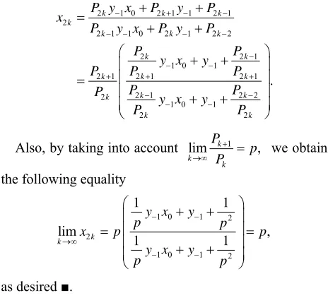
Also, by taking into account _lim k 1 _, k

k

P p P



  we obtain

the following equality

1 0 1 2

2

1 0 1 2

1 1

lim ,

1 1

k k

y x y

p p

x p p

y x y

p p

 



 

 _ _ 

 

 

 _ _ 

 

 

as desired ■.

3. Numerical Examples

In order to illustrate and support theoretical results of the previous section, we consider several examples in this section. These examples represent the qualitative behavior of solutions of the mentioned nonlinear difference equation systems.

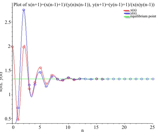
[image:4.595.307.539.271.487.2]

Example 3.1 Consider system (1.3) with the inital conditions x11.5, x03.2, y11.9, y02.3 (See Figure 1).

Example 3.2 Consider system (1.4) with the inital conditions x12.5,x01.2, y10.7, y01.5 (See Figure 2).

4. Conclusion

In this study, we formulated the solutions of equation systems (1.3) and (1.4) and determined their forbidden sets. Obtained formulae are given by means of Padovan numbers. Also, for x1, ,x0 y1,y0F1 and x1, ,x0 y1,y0F2,

(5)

0 5 10 15 20 25 n

0.5 1 1.5 2 2.5

x(

n)

, y(n)

Plot of x(n+1)=(x(n-1)+1)/(y(n)x(n-1)), y(n+1)=(y(n-1)+1)/(x(n)y(n-1))

x

x((nn)) y

y((nn)) e

x n y n

  

1



.

10

5 15 20 25

n

-5

x(

n)

, y(

n)

Plot of x(n+1)=(x(n-1)+1)/(y(n)x(n-1)), y(n+1)=(y(n-1)+1)/(x(n)y(n-1))

x

x((nn))

y

y((nn))

e

x n y n

  

1



.

their equilibrium points and , respec-

tively, where is the plastic number.



,

p p





 p, p



p

REFERENCES

[1] R. P. Agarwal, “Difference Equations and Inequalities,” Marcel Dekker, New York, 2000

[2] M. Aloqeili, “Dynamics of a Rational Difference Equa-tion,” Applied Mathematics and Computation, Vol. 176,

No. 2, 2006, pp. 768-774.

http://dx.doi.org/10.1016/j.amc.2005.10.024

[3] T. F. Ibrahim, “On the Third Order Rational Difference equation

 2 

1

1 2

n n n

x x x

x a bx x  

 



 ,” International Journal of

Contemporary Mathematical Sciences, Vol. 4, No. 25-28,

2009, pp. 1321-1334.

[4] R. Khalaf-Allah, “Asymptotic Behaviour and Periodic

Naturel of Two Difference Equations,” Ukrainian Mathe- matical Journal, Vol. 61, No. 6, 2009, pp. 988-993.

http://dx.doi.org/10.1007/s11253-009-0249-2

[5] E. M. Elabbasy, H. A. El-Metwally and E. M. Elsayed, “Global Behavior of the Solutions of Some Difference Equations,” Advances in Difference Equations, Vol. 2011,

2011, p. 28.

http://dx.doi.org/10.1186/1687-1847-2011-28.

[6] E. M. Elsayed, “Solution and Attractivity for a Rational Recursive Sequence,” Discrete Dynamics in Nature and Society, Vol. 2011, 2011, Article ID: 982309.

[7] C. Cinar, “On the Positive Solutions of the Difference Equation System 1 1

1 1

1

, n

n n

y

x y

y y x

 

 

 

n

,” Applied Mathe-

matics and Computation, Vol. 158, No. 2, 2004, pp. 303-

[image:5.595.103.506.351.505.2]

(6)

Or-der Rational Difference Equations , n p

n n

n p n q n q

by a

x y

y x y



 

 

 ,”

Applied Mathematics and Computation, Vol. 171, No. 2,

2005, pp. 853-856.

[9] A. S. Kurbanli, C. Cinar and I. Yalcinkaya, “On the Be- havior of Positive Solutions of the System of Rational Difference Equations,” Mathematical and Computer Mo- delling, Vol. 53, No.5-6, 2011, pp. 1261-1267.

http://dx.doi.org/10.1016/j.mcm.2010.12.009

[10] E. M. Elsayed, “Solutions of Rational Difference Systems of Order Two,” Mathematical and Computer Modelling,

Vol. 55, No. 3-4, 2012, pp. 378-384. http://dx.doi.org/10.1016/j.mcm.2011.08.012

[11] M. Mansour, M. M. El-Dessoky and E. M. Elsayed, “The Form of the Solutions and Periodicity of Some Systems of Difference Equations,” Discrete Dynamics in Nature and Society, Vol. 2012, 2012, Article ID: 406821.

[12] S. Stevic, “On a System of Difference Equations,” Ap-plied Mathematics and Computation Vol. 218, No. 7,

2011, pp. 3372-3378.

[13] S. Stevic, “On Some Solvable Systems of Difference Equations,” Applied Mathematics and Computation, Vol.

218, No. 9, 2012, pp. 5010-5018.

[14] D. T. Tollu, Y. Yazlik and N. Taskara, “On the Solutions of Two Special Types of Riccati Difference Equation via Fibonacci Numbers,” Advances in Difference Equations,

Vol. 2013, 2013, p. 174.

http://dx.doi.org/10.1186/1687-1847-2013-174

[15] A. S. Kurbanli, C. Cinar and D. Simsek, “On the Perio- dicity of Solutions of the System of Rational Difference

Equations 1 1

1

1 1

n n

1 ₁, ₁

n n

n n n n

x y

y x



 

 



 y x

x y

 



  ,” Applied Mathe-

matics, Vol. 2, No. 4, 2011, pp. 410-413.

http://dx.doi.org/10.4236/am.2011.24050

[16] A. G. Shannon, P. G. Anderson and A. F. Horadam, “Properties of Cordonnier, Perrin and Van der Laan Numbers,” International Journal of Mathematical Educa- tion in Science and Technology, Vol. 37, No. 7, 2006, pp.

825-831.http://dx.doi.org/10.1080/00207390600712554 [17] Benjamin M. M. De Weger, “Padua and Pisa are

Expo-nentially Far Apart,” Publicacions Matematiques, Vol. 41,

No. 2, 1997, pp. 631-651.

http://dx.doi.org/10.5565/PUBLMAT_41297_23